# RACE MODEL APP
# MINIMUM 3 SUBJECTS
# ----------------------------------------------------------
# LOAD PACKAGES
# library(markdown)
library(shiny)
## HELPER FUNCTIONS----
# invert signs
invertSigns <- function(string){
strVector <- strsplit(string,"")[[1]]
s <- paste(sapply(strVector,FUN = function(x) if(x=="+"){"-"}else if(x=="-"){"+"} else {x}),collapse = "")
return(s)
}
# T value calculation
tmax <- function(di)
{
# t-Tests for each percentile
tvalues = rowMeans(di) / apply(di, 1, sd) * sqrt(ncol(di))
#print(tvalues)
# if(anyNA(tvalues)){
# nacount = sum(is.na(tvalues))
# warning(paste0('There were ',nacount,' NaNs of ',length(tvalues),' tvalues of tmax function!'))}
max(tvalues,na.rm = T)
} # tmax
tval <- function(di)
{
# t-Tests for each percentile
tvalues = rowMeans(di) / apply(di, 1, sd) * sqrt(ncol(di))
#print(tvalues)
tvalues
}
pval <- function(tval,n)
{
# calculates pvalues from tvalues
pvalues = pt(tval,df = n-1,lower.tail = FALSE)
}
## random generation functions
## from https://github.com/rforge/lcmix/blob/master/pkg/R/distributions.R
rmvnorm <- function(n, mean=NULL, cov=NULL)
{
## munge parameters PRN and deal with the simplest univariate case
if(is.null(mean))
if(is.null(cov))
return(rnorm(n))
else
mean = rep(0, nrow(cov))
else if (is.null(cov))
cov = diag(length(mean))
## gather statistics, do sanity checks
D = length(mean)
if (D != nrow(cov) || D != ncol(cov))
stop("length of mean must equal nrow and ncol of cov")
E = eigen(cov, symmetric=TRUE)
if (any(E$val < 0))
stop("Numerically negative definite covariance matrix")
## generate values and return
mean.term = mean
covariance.term = E$vec %*% (t(E$vec) * sqrt(E$val))
independent.term = matrix(rnorm(n*D), nrow=D)
drop(t(mean.term + (covariance.term %*% independent.term)))
}
rmvgamma <- function(n, shape=1, rate=1, corr=diag(length(shape)))
{
## extract parameters, do sanity checks, deal with univariate case
if(!is.matrix(corr) || !isSymmetric(corr))
stop("'corr' must be a symmetric matrix")
D = ncol(corr)
Ds = length(shape)
if(Ds > D)
warning("'shape' longer than width of 'corr', truncating to fit")
if(Ds != D)
shape = rep(shape, length.out=D)
Dr = length(rate)
if(Dr > D)
warning("'rate' longer than width of 'corr', truncating to fit")
if(Dr != D)
rate = rep(rate, length.out=D)
if(D == 1) rgamma(n, shape, rate)
## generate standard multivariate normal matrix, convert to CDF
Z = rmvnorm(n, cov=corr)
cdf = pnorm(Z)
## convert to gamma, return
sapply(1:D, function(d) qgamma(cdf[,d], shape[d], rate[d]))
}
## DEFAULT VARIABLES
formatexample<-'
# Obs: Observer/Subject
# Cond: Condition
# RT: Response time (Inf: omitted response)
#
Obs Cond   RT  # Include this header
1    A  245  # Response to A
1    V  281  # Response to V
1   AS  212  # Response to AS
1    V  Inf  # Omitted response to V
# and so on'
## UI --------------------------------------------------------------------
library(markdown)
library(shiny)
ui<-shinyUI(
fluidPage(
includeScript("../../../Matomo-tquant.js"),
# include to render mathjax formular on shiny server
withMathJax(),
# fluidRow(
# # DEVELOPER UI =================================================================================
# checkboxInput("check_dev", label = "development modus", value = F),
# conditionalPanel("input.check_dev",
# h3('Developer Output'),
# fluidRow(column(12,
# #div("more math here \\sqrt{2}"),
# verbatimTextOutput("devoutput")
# # column(12,h1(p(HTML("<a href='#inequality'>Analysis</a>"))))
# ))
# )
# ),
fluidRow(column(12,align='center',
h1('Race Model App')
)),
fluidRow(
navbarPage(" ", # "Race Model Test",
#align='center',
# START PAGE =================================================================================================================================================================
tabPanel('Home',
fluidPage(fluidRow(
column(2),
column(8, #align='center',
p("
We regularly encounter multisensory signals in our daily life. They are often used to increase attention and promote fast responses.
Messenger applications on mobile phones, for instance, usually inform the user about newly arrived messages not only via pop-up icons on the display (visual) but also with short sounds (auditory) or even vibrations (tactile). Studies show that persons who are asked to detect certain target stimuli are often faster, when those stimuli address several sensory modalities compared to only one modality. This phenomenon is called the redundant signals effect. There are different types of models to explain this observation - either with or without multisensory integration.
" ),
p(
'
This application allows you to get familiar with the different models and techniques used to investigate the redundant signals effect.
You can either upload your own data from a redundant stimulus detection experiment (via Get Data>Upload) or simulate data in the simulation section (via Get Data>Simulation). In the next step you can test your uploaded/simulated data for multisensory integration and draw your own conclusions. Below you find a quick tour that guides you through the app.
'
)
),
column(2)
),
fluidRow(column(12,align='center',HTML('<br>'),h3('Quick Start'),HTML('<br>'))),
fluidRow(
column(3),
column(6,
p(''),
p('1. Click the "Get Data" panel in the header.'),
HTML('<p><img src="get_data.png" width="70" /></p>'),
p('2. Choose "Upload" if you have your own data set. Else stay with "Simulation".'),
HTML('<p><img src="upload.png" width="120" /></p>'),
p('2.1 (Simulation:) For now you can leave the default settings unchanged, scroll down and click the "Generate Data" button.'),
HTML('<p><img src="generate.png" width="100" /></p>'),
p('3. Click the "Analysis" panel in the header.'),
HTML('<p><img src="analysis.png" width="70" /></p>'),
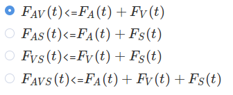
p('4. Select a race model inequality to test. Each inequality tests one redundant stimulation condition, e.g. audio-visual (AV)'),
HTML('<p><img src="rmi_selection.png" width="200" /></p>'),
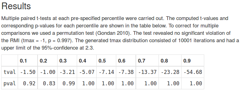
p('5. Inspect the results.'),
HTML('<p><img src="results.png" width="200" /></p>'),
p('6. Is there evidence for multisensory integration in any of the redundant stimulation conditions?')
),
column(3)
),
fluidRow(column(12,align='center',HTML('<br>'),h3('Play with the parameters ...'),HTML('<br><br>'))),
fluidRow(
column(3),
column(6,
p('7. (Simulation:) Go back to the simulation section and change the parameters. To update the new parameter settings press the "Generate Data" button.'),
p('7.1 How do the reaction times change when you change the intensity rates or the count threshold?'),
HTML('<p><img src="poisson_parameter.png" width="200" /> <img src="simulation_plot.png" width="200" /> </p>'),
p('7.2 What happens when you change the underlying models for the redundant stimulation conditions?'),
HTML('<p><img src="model_selection.png" width="200" /></p>'),
p('7.3 Test your modified data by going back to step 2.1 .'),
HTML('<br><br>')
),
column(3)
)
)),
# GET DATA
tabPanel('Get Data',
tags$head( tags$script(src="http://cdn.mathjax.org/mathjax/latest/MathJax.js?config=TeX-AMS_HTML-full", type = 'text/javascript'),
tags$script( "MathJax.Hub.Config({tex2jax: {inlineMath: [['$','$']]}});", type='text/x-mathjax-config')
),
fluidPage(
fluidRow(
column(4,align='right',
h3('Data')
),
column(8,
radioButtons("getdata", label = '',
choices = list("Upload" = 1, "Simulation" = 2),
selected = 2,inline = T)
)),
hr(), #HTML('<hr style="color: blue;">')
# UPLOAD ===========================================================================
conditionalPanel(condition = "input.getdata == 1",
fluidRow(
column(12,
p("Here you can upload data from your own detection time experiment!
The experiment should include stimuli addressing three different sensory modalities: auditory (A), visual (V) and tactile/somato-sensory(S).
For each participant it should contain reaction times (RT) for seven conditions.
There are the three above mentioned single modality conditions (A,V,S) and conditions, where stimuli targeted more than one modality:
audio-visual (AV), audio-somato-sensory (AS), visual-somato-sensory (VS) and the combination of all three audio-visual-somato-sensory (AVS).
The data should be uploaded in a text-file with three columns as shown in the format example.
")
)),
fluidRow(
column(3),
column(6,
h4('Format Example'),
pre(p(formatexample))
),
column(3),
hr()
),
fluidRow(
column(12,align="center",
hr(),
fileInput('file1', '', # 'Choose txt File',
accept=c('text/csv',
'text/comma-separated-values,text/plain',
'.csv'))
)),
fluidRow(column(12,align='center',p('Next Step: Analyse your data by clicking "Analysis" in the header.'))),
# PDF PLOT OUTPUT
fluidRow(column(width = 12,
#h1('Visualization'),
plotOutput("pdf_plot_upload"))
)
),
# SIMULATION =======================================================================
conditionalPanel(condition = "input.getdata == 2",
fluidPage(
fluidRow(
p("
Here you can simulate data of a detection time experiment! The data will include reaction times (RT) for detection tasks in seven conditions:
In the first three conditions target stimuli were presented to either auditory (A), visual (V) or tactile/somato-sensory(S) modality (single stimulation). In the other four conditions, presented stimuli targeted more than one sensory modality (redundant stimulation). These were audio-visual (AV), audio-somato-sensory (AS), visual-somato-sensory (VS) and the combination of all three audio-visual-somato-sensory (AVS) conditions. Below you can adjust the parameters of the data simulation.
"),
hr()
),
#h1("Simulate Data"),
# h3('Settings'),
# USER INPUT
fluidRow(
column(width = 6,
h3('Single Stimulation'),
p("
For each single stimulus condition you can adjust the parameters for the RT generation. Here, we model RTs to be a combination ($RT = D + m$) of a stimulus detection time $D$ and the duration of other processes $m$, e.g. the motor process which executes a button press with a finger.
While the duration of the later processes $m$ are held constant for all subjects and conditions, each subject has her own distribution of detection times $D$ for each condition."),
p(""),
p("
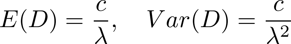
To model the distribution of detection times we use a counter model. According to the counter model, information about a stimulus is continuously accumulated over time. The information arrives as discrete events (counts) which occur one after another. Once their total number exceeds a fixed count threshold, the stimulus is detected. In tasks which require conservative decisions (a minimum of false alarms), the threshold is assumed to be higher compared to tasks which promote liberal decision making. Here the count threshold $c$ is assumed constant over all subjects and conditions. How fast the events occur is characterized by the intensity rate lambda. The higher the intensity rate, the shorter the average time between events.
Together, threshold $c$ and intensity rate lambda determine the detection time $D$, following a gamma distribution with mean and variance:
"),
fluidPage(column(12,align='center',HTML('<p><img src="expD.png" width="200" /></p>'))),
p("To sum up, the higher the intensity rate and the lower the count threshold, the faster the detection time of a person will be."),
p(""),
p("
Below you can adjust the count threshold $c$, the process constant $m$ and the intensity rates lambda on the population level for detection time $D$. The exact individual intensity rates will differ from the population rate with a certain error (see advanced settings) since all persons do not have the same detection time distribution. For a detailed description click the 'Learn more' button at the top.
"),
hr(),
fluidRow(
column(6,
## count c
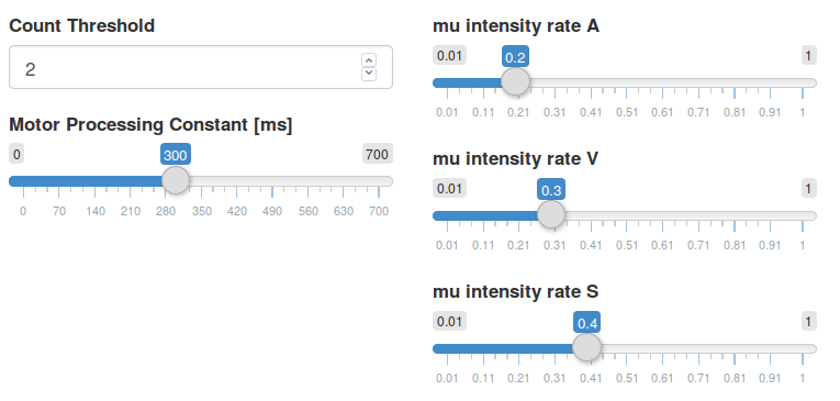
numericInput(inputId = "c", label = "Count Threshold",
value = 2, min = 1, max = 5, step = 1),
## motor constant m
sliderInput("m", label = "Motor Processing Constant [ms]",
min = 0, max = 700, value = 300)
),
column(6,
## intensity rates
#h4("Mu Intensity Rates in Unimodal Conditions"),
sliderInput("A", label = "mu intensity rate A",
min = 0.01, max = 1, value = 0.2),
sliderInput("V", label = "mu intensity rate V",
min = 0.01, max = 1, value = 0.3),
sliderInput("S", label = "mu intensity rate S",
min = 0.01, max = 1, value = 0.4)
)
)
),
column(6,
h3('Redundant Stimulation'),
p("
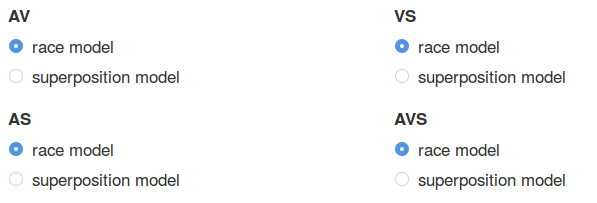
In detection tasks with stimuli addressing more than one sensory modality, subjects tend to show shorter RTs (redundant signals effect). For each redundant condition you can choose whether or not information from different sensory modalities is integrated in order to improve detection speed of stimuli (multisensory integration). Here, as a model of multisensory integration we use Schwarz's (1989) superposition model.
For the case of no multisensory integration occurring, where stimulus processing is carried out separately by each sensory modality, we assume the race model (Raab 1962)."),
p(""),
p("
For the redundant conditions, you do not need to set population intensity rates since those are determined by the parameters for single modality stimulation and the models you select below.
To learn more about the two models have a look at the 'Lean more' section!"
),
hr(),
p('Select the underlying models: with (superposition) or without (race model) multisensory integration'),
fluidRow(
column(6,
radioButtons("radioAV", label = 'AV',
choices = list("race model" = 1, "superposition model" = 2),
selected = 1,inline = F),
radioButtons("radioAS", label = 'AS',
choices = list("race model" = 1, "superposition model" = 2),
selected = 1)),
column(6,
radioButtons("radioVS", label = 'VS',
choices = list("race model" = 1, "superposition model" = 2),
selected = 1),
radioButtons("radioAVS", label = 'AVS',
choices = list("race model" = 1, "superposition model" = 2),
selected = 2))
),
hr(),
h3('Sample Size'),
fluidRow(
column(width = 6,
## number of subj and obs
numericInput(inputId = "nsubj", label = "Number of Subjects (min 3)",
value = 10, min = 3, max = 100, step = 1)
),
column(width = 6,
numericInput(inputId = "nobs", label = "Number of Trials",
value = 200, min = 5, max = 5000, step = 1)
)
)
)),
# ADVANCED INPUT
## checkbox advanced settings
checkboxInput("check_advanced", label = "show advanced settings", value = F), #FALSE),
hr(),
conditionalPanel("input.check_advanced",
h3('Advanced Settings'),
p("Please read the section 'Learn more' before changing these values.
There you will find a detailed description of the (hierarchical) simulation model we used. "),
fluidRow(
## hyper distribution of intensity rates
column(width = 6,
h4('Single Stimulus Intensity Rates'),
p("
The individual intensity rates vary around the population mean intensity rate which you determined above.
Here you can adjust how strongly the individual rates are allowed to differ from the population mean.
Technically, you are changing the standard deviation (SD) of the marginal distributions from the multivariate hyperdistribution (multivariate gamma).
The chosen SD will be the same for all marginals of single stimulus conditions."),
sliderInput(inputId = "sd_lambda", label = "Standard Deviation of Marginal Distributions of Population Intensity Rates",
value = .01, min = 0.001, max = 0.4),
p("We implemented the idea that some subjects are overall faster (high intensity rates) or overall slower (low intensity rates) in detecting stimuli in all sensory modalities. Therefore, the intensity rates for single stimulation conditions A, V, S are positively correlated across subjects. In our simulation this is achieved by drawing individual intensity rates from the above mentioned multivariate hyperdistribution (multivariate gamma) with a positive correlation matrix.
The chosen correlation will be the same between any pair of two intensity rates of single stimulus conditions (hence all off-diagonal elements in the correlation matrix are equal)."),
sliderInput(inputId = "corr_lambda", label = "Correlation of Single Stimulus Intensity Rates over Subjects",
value = .8, min = 0, max = 1)
),
## Correlation Unimodal RT
column(width = 6,
h4("Optimize Race Model"),
p("
Imagine a bicycle race of two opponents at which always only the winner's time would be recorded. Let us say the cyclists have good and bad days which affect their performance. If it were the case that, whenever cyclist 1 has a good day cyclist 2 has a bad day and vice versa, it would be quite rare that both show a poor performance on the same day. Therefore, the average winning time would improve, since slow winning times become rare. The same mechanism is true for the race model.
If the detection times of two 'competing' sensory modalities are negatively correlated, the RTs for redundant conditions become even shorter.
"),
p(""),
p("
For race models with only two sensory modalities the fastest RTs for redundant stimuli are generated by the maximal negative correlation possible. However, in a situation with three 'competing' modalities we do not only have one but three correlation coefficients which leads to a slightly more complicated situation. For three modalities, finding the 'optimal' setting of correlation coefficients is not as trivial as in the two-modality case above. Plus, the correlation coefficients of pairwise correlations between three variables underlie certain upper and lower bounds.
Below you can play around with the correlations and investigate for yourself.
"),
sliderInput("corrAV",
label=HTML("$$ corr~({RT}_A,{RT}_V) $$"),step= 0.1,
min = -0.95, max = 0.95, value = -0.5),
sliderInput("corrAS",
label=HTML("$$ corr~({RT}_A,{RT}_S) $$"),step= 0.1,
min = -0.95, max = 0.95, value = -0.5),
sliderInput("corrVS",
label=HTML("$$ corr~({RT}_V,{RT}_S) $$"),step= 0.1,
min = -1, max = 1, value = -0.5)
)
)
),
# ACTION BUTTON
#hr(),
fluidRow(
column(12,align="center",
actionButton("submit", label = "Generate Data")),
hr()
),
fluidRow(column(12,align='center',HTML('<br>'),p('Next Step: Analyse your data by clicking "Analysis" in the header.'))),
# PDF PLOT OUTPUT
fluidRow(column(width = 12,
#h1('Visualization'),
plotOutput("all_pdf_plot"))
),
fluidRow(column(width = 12, align='center',
selectizeInput(
'selectSubjSim', 'Display Single Subject',
choices = c(as.character(1:10),'all')
)
)),
fluidRow(column(width = 12, align='center',
hr(),
p('You can download the simulated data.
Make sure to open the shiny app in your browser instead of the Rstudio Viewer.
The Viewer appears to have problems with saving files.'),
downloadButton('downloadData', 'Download Generated Data'),
hr()
))
))
)),
# ANALYSIS =================================================================================
tabPanel("Analysis",
fluidPage(
fluidRow(
hr(),
p("
Test the data for multisensory integration. Often there is an improvement in detection time for stimuli which elicit more than one sensory modality (redundant conditions).
Here you can test if faster reaction times (RT) can be explained by a simple race model. If not, we have to assume a model with multisensory integration occurring. As explained in the 'Learn More' section, there are several race model inequalities (RMI) that describe the relations of RT distributions under different conditions in a race model. Is a RMI violated, the corresponding race model has to be rejected and we assume a model with multisensory integration occurring. Each RMI is associated with a certain race model, e.g. the first RMI below refers to a race between auditory and visual detection processes. The last seven RMIs correspond to races between audio, visual and somato-sensory detection processes. Please note, that the last three RMIs can only be tested if the first three RMIs hold. For further explanation see the 'Learn More' section.
"),
checkboxInput("check_method", label = "Check to read more about the used methods", value = F), #FALSE),
conditionalPanel("input.check_method",
h3('Method'),
p("
This is a brief glance at the algorithm used. For a given RMI multiple paired $t$-tests are carried out. They test the alternative hypothesis whether the left hand side of a RMI is greater than the right hand side. The $t$-tests are run at the chosen percentiles $(0.1, 0.2, ...)$ of individual RT distributions. For every percentile each subject contributes estimated density scores, e.g $F_{AV}(t), F_A(t), F_V(t)$, for the associated conditions. After deriving both sides of the RMI, their difference, e.g $F_{AV}(t)−[F_A(t)+F_V(t)]$, is computed for each subject. Paired $t$-tests probe whether the differences are significantly greater than zero across participants. Since there are many $t$-tests for many percentiles, there is a potential of type-I-error inflation. To correct for this we used the permutation test described by Gondan (2010). The test uses the maximum $t$-value of all percentiles, $t_{max}$, as a combined test statistic for a 'global' test. By randomly switching the signs of the individual differences for a large number of iterations, a distribution of tmax under the null-hypothesis is generated.
If the empirical $t_{max}$ statistic lies within the upper 0.05 percentile of the generated distribution, we assume a significant overall violation of the RMI.
"),
hr()
)
),
## Inequality Selection
fluidRow(
column(6,
h3('Select Race Model Inequality'),
radioButtons('inequality', '' #'Choose Inequality to test'
,c( '$F_{AV}(t) $<=$ F_A(t) + F_V(t)$' = 'FAV()-FA()-FV()'
,'$F_{AS}(t) $<=$ F_A(t) + F_S(t) $' = 'FAS()-FA()-FS()'
,'$F_{VS}(t) $<=$ F_V(t) + F_S(t) $' = 'FVS()-FV()-FS()'
,'$F_{AVS}(t) $<=$ F_A(t) + F_V(t) + F_S(t) $' = 'FAVS()-FA()-FV()-FS()'
,'$F_{AVS}(t) $<=$ F_{AV}(t) + F_S(t) $' = 'FAVS()-FAV()-FS()'
,'$F_{AVS}(t) $<=$ F_{AS}(t) + F_V(t) $' = 'FAVS()-FAS()-FV()'
,'$F_{AVS}(t) $<=$ F_{VS}(t) + F_A(t) $' = 'FAVS()-FVS()-FA()'
,'$F_{AVS}(t) $<=$ F_{AV}(t) + F_{AS}(t) - F_A(t) $' = 'FAVS()-FAV()-FAS()+FA()'
,'$F_{AVS}(t) $<=$ F_{AV}(t) + F_{VS}(t) - F_V(t) $' = 'FAVS()-FAV()-FVS()+FV()'
,'$F_{AVS}(t) $<=$ F_{AS}(t) + F_{VS}(t) - F_S(t) $' = 'FAVS()-FAS()-FVS()+FS()'
#,'Minimum of last three upper bounds:' = 'FAVS()-min(FAV()+FAS()-FA(),FAV()+FVS()-FV(),FAS()+FVS()-FS())'
)
# ,'$F_{AVS}(t) $<=$ ~ min[F_{AV}(t) + F_{AS}(t) - F_A(t), F_{AV}(t) + F_{VS}(t) - F_V(t),F_{AS}(t) + F_{VS}(t) - F_S(t)]$' = 'FAVS()-min(FAV()+FAS()-FA(),FAV()+FVS()-FV(),FAS()+FVS()-FS())')
, selected = NULL, inline = F, width = NULL
),
#fluidPage(column(12,align='left',HTML('<p><img src="minRMI.png" width="335" /></p>'))),
## Flexible Percentiles
h3('Select Percentiles'),
p('Select percentiles at which $t$-tests will be carried out. Race model violations are more likely to occur at lower percentiles.
Hence restricting the tests to lower percentiles might increase the overall significance.
'),
# sliderInput("range", "Select percentiles at which t-tests will be carried out",
# min = 0.05, max = 0.95, value = c(0,1),step = 0.05)
sliderInput("range", "",
min = 0.1, max = 0.9, value = c(0,1),step = 0.1)
),
column(6, align='center',
## CDF Plots
plotOutput('plot_cdf_ineq'),
## Select Subject
selectizeInput(
'selectSubjAna', 'Display Single Subject',
choices = c('all',as.character(1:10))
)
)
),
## Results
fluidRow(
hr(),
h3('Results'),
textOutput('permtext')
),
fluidRow(column(12,align='center',HTML('<br>'),tableOutput('tvalues_table')))
)
),
# THEORY ========================================================================================================================
tabPanel('Learn more',
fluidPage(
fluidRow(align='center',
#'Please activate your in-browser pdf viewer to display text.',
# tags$iframe(style="height:800px; width:100%; scrolling=yes",
# src="theory_section_3_graf.pdf")
HTML('<p><img src="learn_more.png" width=80% /></p>')
# HTML('<p><img src="1.png"/></p>'),
# HTML('<p><img src="2.png"/></p>'),
# HTML('<p><img src="3.png"/></p>'),
# HTML('<p><img src="4.png"/></p>'),
# HTML('<p><img src="5.png"/></p>'),
# HTML('<p><img src="6.png"/></p>')
)
))
#ABOUT ===========================================================================================================================
,
tabPanel('About',
fluidPage(
column(10, #align='center',
p("This web application was created during the ",a("TquanT initiative", href='https://tquant.eu/' )," to promote quantitative thinking.
The app provides a tool to learn statistical techniques in an interactive environment."),
h4('Team'),
p("Felix Wolff, Department of Psychology, Carl von Ossietzky Universitaet Oldenburg, Oldenburg, Germany"),
p("email: felix.wolff[at]uol.de"),
p("Prof. Dr. Hans Colonius, Department of Psychology, Carl von Ossietzky Universitaet Oldenburg, Oldenburg, Germany")
)
))
)
)
)
)
## SERVER --------------------------------------------------------------------
server<-shinyServer(function(input, output,session) {
# DEFAULT SETTINGS
## simulation
### sigma lambda
SIGMA_LAMBDA <- reactive({
rho <- input$corr_lambda
M = matrix(rho,ncol = 3,nrow = 3)
diag(M) = c(1,1,1)
M
})
## analysis
# q <- reactive(seq(input$range[1], input$range[2], by=0.05)) #seq(0, 1, by=.1) #
q <- reactive(seq(input$range[1], input$range[2], by=0.1))
nperm=1001
### sigma uni T (unimodal arrival times)
SIGMA_UNI_T <- reactive({
corrAV <- input$corrAV
corrAS <- input$corrAS
corrVS <- input$corrVS
array(c(1,corrAV,corrAS,
corrAV,1,corrVS,
corrAS,corrVS,1),dim=c(3,3))
})
## graphical settings
RT_LABELS = c('RT_A','RT_V','RT_S','RT_AV','RT_AS','RT_VS','RT_AVS')
CONDITIONS = c('A','V','S','AV','AS','VS','AVS')
COLORS_DARK = c('dodgerblue4','firebrick4','yellow3','orchid4','green4','darkorange3','gray8')
COLORS_BRIGHT = c('dodgerblue2','firebrick2','yellow1','orchid2','green2','darkorange1','gray52')
COLOR_SCHEME <- COLORS_BRIGHT
# DATA UPLOAD SERVER ====================================================================================
# read in data
DATA_UP <- reactive({
inFile <- input$file1
if (is.null(inFile))
return(NULL)
dat<-read.table(inFile$datapath, header=T)
Obs = split(dat[, c('Cond', 'RT')], dat$Obs)
lapply(Obs, function(x) split(x$RT, x$Cond))
})
# plot uploaded RT
output$pdf_plot_upload <- renderPlot({
if (is.null(DATA_UP()))
return(NULL)
## plot parameters
QUAN_UP = quantile(unlist(DATA_UP()),probs = c(.01,.99))
maxdens <- max(sapply(DATA_UP(),function(s) max(density(s$AVS)$y)))
upload_title <- 'Smoothed Histogram of RT for all Subjects'
XLIMITS_UP = QUAN_UP + c(-2,2) # c(200,800)
YLIMITS_UP = c(0,maxdens)
plot(x=NA,xlim=XLIMITS_UP,ylim = YLIMITS_UP,ylab = '',xlab = 'RT (ms)',bty='n', main=upload_title) # empty plot
for(s_idx in 1:length(DATA_UP())){
for(c_idx in 1:length(CONDITIONS)){
lines(density(DATA_UP()[[s_idx]][[CONDITIONS[c_idx]]]),col=COLOR_SCHEME[c_idx] ,lwd=1)
}
}
legend(x=diff(XLIMITS_UP)*0.8 + XLIMITS_UP[1], y=YLIMITS_UP[2],#x = quan95-5, 0.4,#y = YLIMITS[2]*0.9, # 310,0.4,
legend = CONDITIONS,col = COLOR_SCHEME,lty=1,bty = 'n',lwd = 1.5)
})
# Some very basic summary statistics
output$summary <- renderTable({
if (is.null(DATA_UP()))
return(NULL)
md = function(x) median(x[x < Inf])
mn = function(x) mean(x[x < Inf])
pc = function(x) 100*mean(x < Inf)
Median = rowMeans(sapply(DATA_UP(), function(x) sapply(x, md)))
Mean = rowMeans(sapply(DATA_UP(), function(x) sapply(x, mn)))
`Detect%` = rowMeans(sapply(DATA_UP(), function(x) sapply(x, pc)))
round(rbind(Median, Mean, `Detect%`))
})
# DATA SIMULATION SEVER ==================================================================================----
# ADVANCED SETTINGS
## advanced settings dynmaical input
observe({
corrAV <- input$corrAV
corrAS <- input$corrAS
updateSliderInput(session, "corrVS",
#label = HTML("$$ corr~(RT_V,RT_S) $$"),
min = ceiling(10*(corrAV*corrAS - sqrt((corrAV^2-1)*(corrAS^2-1))))/10,
max = floor(10*(sqrt((corrAV^2-1)*(corrAS^2-1)) + corrAV*corrAS))/10,
step= 0.1,
value = input$corrVS
)
})
# GENERATE DATA ON BUTTON CLICK
DATA_SIM<- eventReactive(input$submit,{
if(input$nsubj<3){
warning("Number of subjects must be 3 or higher!")
return(NULL)
}
## user input
nsubj = input$nsubj
nobs = input$nobs
m = input$m
c = input$c
MU_LAMBDA <- c(input$A,input$V,input$S)
INPUT_SUMMARY = list(nsubj=nsubj,nobs=nobs,m=m,c=c,MU_LAMBDA=MU_LAMBDA)
v_lambda = (input$sd_lambda)^2
## indivdual lambdas
### reparametrize gamma parameters
S = MU_LAMBDA^2/v_lambda
R = MU_LAMBDA/v_lambda
LAMBDAS <- rmvgamma(n = nsubj,shape = S,rate = R, corr = SIGMA_LAMBDA())
colnames(LAMBDAS) <- c('A','V','S')
## unimodal reaction times RT
RT_UNI = array(data = NA,dim = c( nsubj, nobs,3))
dimnames(RT_UNI)[[3]] <- c('A','V','S')
for (i in 1:nsubj){
RT_UNI[i,,] = rmvgamma(n = nobs,shape = c,rate = LAMBDAS[i,],corr = SIGMA_UNI_T()) + m
}
## bimodal reaction times
### AV
if(input$radioAV == 1){
RT_AV = apply(RT_UNI[,,c('A','V')],c(1,2),min)
}else{
RT_AV = array(data = NA,dim = c(nsubj,nobs))
for (i in 1:nsubj){
RT_AV[i,] = rgamma(n = nobs,shape = c,rate = sum(LAMBDAS[i,c('A','V')])) + m
}
}
### AS
if(input$radioAS == 1){
RT_AS = apply(RT_UNI[,,c('A','S')],c(1,2),min)
}else{
RT_AS = array(data = NA,dim = c(nsubj,nobs))
for (i in 1:nsubj){
RT_AS[i,] = rgamma(n = nobs,shape = c,rate = sum(LAMBDAS[i,c('A','S')])) + m
}
}
### VS
if(input$radioVS == 1){
RT_VS = apply(RT_UNI[,,c('V','S')],c(1,2),min)
}else{
RT_VS = array(data = NA,dim = c(nsubj,nobs))
for (i in 1:nsubj){
RT_VS[i,] = rgamma(n = nobs,shape = c,rate = sum(LAMBDAS[i,c('V','S')])) + m
}
}
## trimodal arrival times and reaction times
### AVS
if(input$radioAVS == 1){
RT_AVS = apply(RT_UNI[,,c('A','V','S')],c(1,2),min)
}else{
RT_AVS = array(data = NA,dim = c(nsubj,nobs))
for (i in 1:nsubj){
RT_AVS[i,] = rgamma(n = nobs,shape = c,rate = sum(LAMBDAS[i,c('A','V','S')])) + m
}
}
## return DATA
RT <-list(
A = RT_UNI[,,'A'],
V = RT_UNI[,,'V'],
S = RT_UNI[,,'S'],
AV=RT_AV,
AS=RT_AS,
VS=RT_VS,
AVS=RT_AVS)
DATA_SIM<- list(INPUT_SUMMARY=INPUT_SUMMARY,RT=RT)
})
Test <- 'test'
# DOWNLOAD DATA
## transform to SIM_DATA from list to data.frame format
DATA_FRAME <- reactive({
data <- d()
nsubj <- length(data)
ncond <- 7
RT <- unlist(data)
nRT <- length(data[[1]][[1]])
Cond <- rep(rep(names(data[[1]]),each=nRT),nsubj)
Obs <- rep(1:nsubj,each=ncond*nRT)
DATA <-data.frame(Obs, Cond, RT)
})
output$downloadData <- downloadHandler(
filename = function() {
#paste0('simulated_rt_racemodel', '.txt')
'simulated_rt_racemodel.txt'
},
content = function(file) {
write.table(DATA_FRAME(), file,quote = F,row.names = F)
}
)
# RT GRAPHICAL OUTPUT
output$all_pdf_plot <- renderPlot({
## return NULL if dependencies are NULL
if(is.null(DATA_SIM()) | input$selectSubjSim==""){
return(NULL)
}
## plot parameters
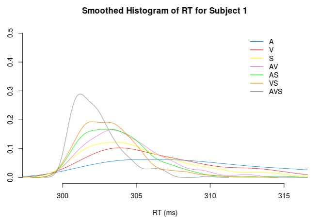
quan95 = quantile(unlist(DATA_SIM()$RT[CONDITIONS]),probs = .95)
XLIMITS = c(DATA_SIM()$INPUT_SUMMARY$m,quan95) + c(-2,2) #c(0,1000) # reactive(c(input$m 50 ,1000))
YLIMITS = c(0,0.5)
## input parameters
if (input$selectSubjSim == 'all')
{
SUBJ = 1:length(d())
}else{
SUBJ = as.numeric(input$selectSubjSim)
}
## plot title
if(input$selectSubjSim=='all'){
simtitle <- 'Smoothed Histogram of RT for all Subjects'
}else{
simtitle <- paste0('Smoothed Histogram of RT for Subject ',input$selectSubjSim)
}
## empty plot
plot(x=NA,xlim=XLIMITS,ylim = YLIMITS,ylab = '',xlab = 'RT (ms)',bty='n', main = simtitle)
for(cond in 1:length(CONDITIONS)){
# plot individual RT
for (i in SUBJ){
lines(density(DATA_SIM()$RT[[CONDITIONS[cond]]][i,]),col=COLOR_SCHEME[cond] ,lwd=1)
}
}
legend(x=diff(XLIMITS)*0.8 + XLIMITS[1], y=YLIMITS[2],#x = quan95-5, 0.4,#y = YLIMITS[2]*0.9, # 310,0.4,
legend = CONDITIONS,col = COLOR_SCHEME,lty=1,bty = 'n',lwd = 1.5
)
})
## display single subjects
observe({
updateSelectInput(session, "selectSubjSim",
choices = c(as.character(1:length(d())),'all')
)
})
# ANALYSIS SERVER ==================================================================================----
# SELECT UPLOADED OR SIMULATED DATA
d <- reactive({
## upload selected
if(input$getdata == 1){
D<-DATA_UP()
}
## simulation selected
if(input$getdata == 2){
### DATA_SIM() empty?
if(is.null(DATA_SIM())){
warning("DATA_SIM() is null!")
return(NULL)
}
### transform simdata into analysis format
### data$RT$cond: nsubj x obs --> data$nsubj$cond
subj_idx <- 1:dim(DATA_SIM()$RT[[1]])[1]
cond_idx <- 1:length(DATA_SIM()$RT)
D<-lapply(subj_idx, function(subj_idx) lapply(cond_idx, function(cond_idx) DATA_SIM()$RT[[cond_idx]][subj_idx,]))
for(i in 1:length(D)){names(D[[i]])<- names(DATA_SIM()$RT)}
}
D
})
# output$listview <- renderPrint({
# str(d())
# })
# Determine quantiles from entire set of response times
rt <- reactive({
tmix <- lapply(d(), unlist)
lapply(tmix, function(x) quantile(x[x < Inf], q()))})
# Evaluate distribution functions at t
FA <- reactive({ mapply(function(ti, qi) ecdf(ti$A)(qi), d(), rt()) })
FV <- reactive({ mapply(function(ti, qi) ecdf(ti$V)(qi), d(), rt()) })
FS <- reactive({ mapply(function(ti, qi) ecdf(ti$S)(qi), d(), rt()) })
FAV <- reactive({ mapply(function(ti, qi) ecdf(ti$AV)(qi), d(), rt()) })
FAS <- reactive({ mapply(function(ti, qi) ecdf(ti$AS)(qi), d(), rt()) })
FVS <- reactive({ mapply(function(ti, qi) ecdf(ti$VS)(qi), d(), rt()) })
FAVS <- reactive({ mapply(function(ti, qi) ecdf(ti$AVS)(qi), d(), rt()) })
## permutation t-tests
# calculate differences
di <- reactive({
mat <- eval(parse(text=input$inequality))
# mat <- eval(parse(text='FAV()-FA()-FV()'))
matrix(mat, nrow=length(q()), ncol=length(d())) })
inequalityString <-reactive({input$inequality})
output$permtext <- renderText({
if(is.null(d())){
return(NULL)
}
stat = tmax(di()) # observed test statistic
# permutation distribution of test statistic
stati = numeric(nperm)
for(i in 1:nperm)
stati[i] = tmax(di() %*% diag(sign(rnorm(d()))))
pval <- mean(stat <= stati)
conf <- quantile(stati, probs=0.95)
inequalityString=input$inequality
if(pval<0.05){
conclusion_bool <- 'a'
conclusion_part1 <- 'Hence, we assume an alternative "coactivation model" for the selected '
conclusion_part2 <-'condition, where some kind of integration of the activation from the different stimulus modalities takes place.'
}else{
conclusion_bool <- 'no'
conclusion_part1 <- 'Hence, we do not need to assume an alternative "coactivation model" for the selected '
conclusion_part2 <-'condition, where some kind of integration of the activation from the different stimulus modalities would take place.'
}
paste0(" Multiple paired t-tests at each pre-specified percentile were carried out.
The computed t-values and corresponding p-values for each percentile are shown in the table below.
To correct for multiple comparisons we used a permutation test (Gondan 2010). The test revealed ",conclusion_bool," significant violation of the RMI (tmax = ",round(stat,2),
", p = ",round(pval,3),
"). ",conclusion_part1,conclusion_part2) #The generated tmax distribution consisted of ",nperm," iterations and had a upper limit of the 95%-confidence at ",round(conf,2),".")
})
# observed paired t-tests
output$tvalues_table <- renderTable({
if(is.null(d())){
return(NULL)
}
tvals <- tval(di())
pvals <- pval(tvals,ncol(di()))
mat <- as.matrix(cbind(tvals,pvals))
colnames(mat)<-c('tval','pval')
rownames(mat)<-q()
res <-t(mat)
res
})
## Plot Inequality CDFs
## display single subjects
observe({
updateSelectInput(session, "selectSubjAna",
choices = c(as.character(1:length(d())),'all')
)
})
output$plot_cdf_ineq <- renderPlot({
if(is.null(d()) | input$selectSubjAna==""){
return(NULL)
}
## axes limits
rthigh <- max(unlist(rt()))
rtlow <- min(unlist(rt()))
xlim <- c(rtlow,rthigh)
ylim <- c(0,1)
## split difference string, e.g. "FAVS()-FVS()-FA()" --> "FAVS()", "FVS()-FA()"
s1 <- sub(x =inequalityString(),pattern = '-',replacement = "SPLIT" ) # sub first minus with SPLIT
s2 <- strsplit(x = s1, split = "SPLIT")[[1]]
ineqleftstring <- s2[1]
ineqrightstring <- invertSigns(s2[2]) # invert minus and plus
## calculate sides
ineqright <- eval(parse(text=ineqrightstring))
ineqleft <- eval(parse(text=ineqleftstring))
# plot
## input parameters and plot title
if (input$selectSubjAna == 'all')
{
SUBJ = 1:length(d())
anatitle <- 'Empirical Cumulative Distribution Function of RT in Redundant Condition \n against Upper Race Model Boundary for all Subjects'
}else{
SUBJ = as.numeric(input$selectSubjAna)
anatitle <- paste0('Empirical Cumulative Distribution Function of RT in Redundant Condition \n against Upper Race Model Boundary for Subject ',input$selectSubjAna)
}
## empty plot
plot(1, main=anatitle, xlab="RT (ms)", ylab="cumulative density"
,type="n", axes=T,xlim = xlim,ylim=ylim,bty='n')
par(new=T)
for (s in SUBJ){
matplot(rt()[[s]]
,cbind(ineqleft[,s],ineqright[,3])
# ,cbind(FA[,s],FV[,s],FS[,s],FAV[,s],FAS[,s],FVS[,s],FAVS[,s])
,type = 'l', lty=1,ylim = ylim,xlim=xlim,axes=F,xlab='',ylab=''
,col=c(1:2))
par(new=T)
}
# legend
ineqsides <- c(gsub(x = ineqleftstring,pattern = "()",replacement = "",fixed = T), # remove brackets
gsub(x = ineqrightstring,pattern = "()",replacement = "",fixed = T))
legend("bottomright", inset=.05, legend=ineqsides, lty=1, col=c(1:length(ineqsides)), horiz=F,bty='n')
par(new=F)
#abline(h=1)
})
# DEVELOPEMENT OUTPUT ==============================================================
output$devoutput <- renderPrint({
require(pastecs)
# QUAN_UP <- reactive(quantile(unlist(DATA_UP()[CONDITIONS]),probs = c(.05,.95))),
# XLIMITS_UP = QUAN_UP() + c(-2,2)
# QUAN_UP = quantile(unlist(DATA_UP()),probs = c(.05,.95))
# if (input$selectSubjAna == 'all')
# {
# SUBJ = 1:length(d())
# }else{
# SUBJ = as.numeric(input$selectSubjAna)
# }
#
# data <- DATA_SIM()$RT
# RT <- unlist(data)
out=list(
# d=str(d()),
# DATA_UP=names(DATA_UP()),
# DATA_SIM=dim(DATA_SIM()$RT[[1]]),
# choice = input$getdata
# quan= quantile(unlist(DATA_UP()[CONDITIONS]),probs = c(.05,.95))
# maxdens = maxdens
# QUAN_UP=QUAN_UP
#l=length(d()),
#choice= input$selectSubjAna,
# SUBJ = SUBJ,
# nulltest=(is.null(d()) | input$selectSubjAna=="")
#dataframe = DATA_FRAME()
# simdata = DATA_SIM()$RT
d=d()
# nsubj = input$nsubj
#percentiles = input$range,
#seqence = seq(input$range[1], input$range[2], by=0.1)
)
out
})
})
shinyApp(ui = ui, server = server)