TWIN Model

The Time-Window of Integration Model (TWIN)

This Shiny App helps you to learn about the Time-Window of Integration Model (TWIN), developed by Hans Colonius, Adele Diederich, and colleagues (Colonius & Diederich, 2004).

It allows you to visualize model predictions, simulate data, and estimate the model parameters either from simulated data or from your own datafile.

This project is part of

Paradigms

Experimental Setup

Crossmodal condition:

Two (or more) stimuli are presented in different modalities simultaneously or with a short delay (stimulus-onset asynchrony) between the stimuli.

Unimodal condition:

One stimulus is presented in one modality.

Participant's Task

... depends on the paradigm.

Focused Attention Paradigm (FAP)

Respond as quickly as possible to a stimulus of a pre-defined modality (target) and ignore the other stimulus (non-target modality).

In the following we assume that the visual stimulus is the target modality, and the auditory stimulus is the non-target modality.

Redundant Target Paradigm (RTP)

Respond to a stimulus of any modality detected first.

Hypothesis

Multisensory integration of sensory information into a perceptual unit (event) occurs only if the peripheral sensory processes all terminate within a given temporal interval, the Time-Window of Integration.

First Stage Assumption

The first stage consists in a (stochastically independent) race among the peripheral processes in the visual and auditory pathways triggered by a crossmodal stimulus complex.

Second Stage Assumption

The second stage comprises all processes following the first stage including preparation and execution of a response.

Time-Window of Integration Assumption

Multisensory integration occurs only if the peripheral processes of the first stage all terminate within a given temporal interval, the time window of integration.

Assumption of Temporal Separability

The amount of interaction, manifesting itself in an increase or decrease of second stage processing time, is a function of crossmodal stimulus features, but it does not depend on the presentation asynchrony (SOA) of the stimuli.

Reaction Times

The total reaction time in the crossmodal condition ($RT_{VA})$ is the sum of the processing times in stage 1 and stage 2. Let $M1$ and $M2$ denote two random variables that refer to the first and second stage processing times, so that the overall reaction time becomes $$RT_{VA} = M_1 + M_2.$$

$I$ is the event that multisensory integration occurs, with probability $P(I)$.
$E[M_2|\neg I]$ is the expected stage 2 processing time conditioned on multisensory integration not occuring.
$\Delta$ is the size of the crossmodal interaction effect.

Expected reaction times for the crossmodal condition:

$$E[RT_{VA}] = E[M_1] + E[M_2|\neg I] - P(I) \cdot \Delta$$

See derivation

$$\begin{align} E[RT_{VA}] &= E[M_1] + E[M_2] \\ &= E[M_1] + P(I) \cdot E[M_2|I] + (1-P(I)) \cdot E[M_2|\neg I] \\ &= E[M_1] + E[M_2|\neg I] - P(I) \cdot (E[M_2|\neg I] - E[M_2|I]) \\ &= E[M_1] + E[M_2|\neg I] - P(I) \cdot \Delta \end{align}$$ with $\Delta \equiv E[M_2|\neg I] - E[M_2|I]$

Expected reaction times for the unimodal conditions:

$$E[RT_{V}] = E[V] + E[M_2|\neg I]$$

Random Variable Distributions

First Stage

Random variable $M_1$ refers to the peripheral processing time in stage 1. For the processing times for the visual and the acoustic stimulus, V and A denote the two statistically independent, exponentially distributed random variables.

See density functions

The density functions are then $$\begin{align} f_V(t) = \lambda_{V}e^{-\lambda_{V}t} \\ f_A(t) = \lambda_{A}e^{-\lambda_{A}t} \end{align}$$ for $t \geq 0$, and $f_V(t) = f_A(t) \equiv 0$ for $t<0.$ The corresponding distribution functions are $F_V(t)$ and $F_A(t)$, respectively.

Second Stage

Random variable $M_2$ refers to the processing time in stage two and is assumed to be normally distributed with mean $\mu - \Delta$ in the crossmodal condition and mean $\mu$ in the unimodal condition.

Expected Reaction Times

Expected reaction times for the crossmodal condition:

Focused Attention Paradigm (FAP)

$$ E[RT_{VA}] = \tfrac{1}{\lambda_V} + \mu - P(I_{FAP}) \cdot \Delta$$

Redundant Target Paradigm (RTP)

$$E[RT_{VA}] = E[min(V,A)] + \mu - P(I_{RTP}) \cdot \Delta$$

Expected reaction times for the unimodal condition:

$$\begin{align} E[RT_V] = \tfrac{1}{\lambda_V} + \mu \end{align}$$

Probability of Integration

The occurrence of multisensory integration depends on the first stage processing times $V$ and $A$, the stimulus onset asynchrony (SOA, denoted by $\tau$), and the width of the Time-Window of Integration, denoted by $\omega$.

The SOA is defined such that the visual stimulus is always presented at $\tau = 0$. Thus, $\tau > 0$ indicates that that the visual is presented before the auditory stimulus, and $\tau < 0$ indicates the reverse presentation order.

For the different paradigms, the event of multisensory integration is defined somewhat differently.

Focused Attention Paradigm

For FAP, the event of multisensory integration is defined as $$I_{FAP} = \{A + \tau < V < A + \tau + \omega\}.$$ The probability of integration can therefore be calculated as $$\begin{align} P(I_{\tau, \omega}) &= P(A + \tau < V < A + \tau + \omega) \\ &= \int_{0}^{\infty} \! f_A(x)\{F_V(x + \tau + \omega) - F_V(x+\tau)\}\,\mathrm{d}x \end{align}$$ where the solutions of the integral depend on the sign of $\omega$ + $\tau$. See solutions of the integral.

(i) $\tau$ < $\tau$ + $\omega$ < 0 $$\begin{align} P(I_{\tau,\omega}) &= \int_{-\tau-\omega}^{-\tau} \! \lambda_{A}e^{-\lambda_{A}x}{1-e^{-\lambda_V(x+\tau+\omega)}} \, \mathrm{d}x -\int_{-\tau}^{\infty} \! \lambda_{A}e^{-\lambda_{A}x}{e^{-\lambda_V(x+\tau)} - e^{-\lambda_V(x+\tau+\omega)}} \, \mathrm{d}x \\ &= \frac{\lambda_V}{\lambda_V+\lambda_A} e^{\lambda_A\tau} (-1 + e^{\lambda_A\omega}); \end{align}$$ (ii) $\tau$ < 0 < $\tau$ + $\omega$ $$\begin{align} P(I_{\tau,\omega}) &= \int_{0}^{-\tau} \! \lambda_{A}e^{-\lambda_{A}x}\{1-e^{-\lambda_V(x+\tau+\omega)}\} \, \mathrm{d}x + \int_{-\tau}^{\infty} \! \lambda_{A}e^{-\lambda_{A}x}\{e^{-\lambda_V(x+\tau)} - e^{-\lambda_V(x+\tau+\omega)}\} \, \mathrm{d}x \\ &= \frac{1}{\lambda_V+\lambda_A} \{\lambda_A(1-e^{-\lambda_V(\omega+\tau)})+ \lambda_V(1-e^{\lambda_A\tau})\}; \end{align}$$ (iii) $0 < \tau < \tau + \omega$ $$\begin{align} P(I_{\tau,\omega}) &= \int_{0}^{\infty} \! \lambda_{A}e^{-\lambda_{A}x}\{e^{-\lambda_V(x+\tau)} - e^{-\lambda_V(x+\tau+\omega)}\} \, \mathrm{d}x \\ &= \frac{\lambda_A}{\lambda_V+\lambda_A} \{e^{-\lambda_V(\tau)}-e^{-\lambda_V(\omega+\tau)}. \end{align}$$

Redundant Target Paradigm

For RTP, multisensory integration occurs only in two events, which are united in $$I_{RTP} = \{A + \tau < V < A + \tau + \omega\} \cup \{V < A + \tau < V + \omega\},$$ The probability of integration $P(I_{RTP})$ is computed as the sum of the probabilities of the two events above, $P(I_{RTP}) = p_1 + p_2$. In the first case, the acoustic stimulus wins the race in the first stage: $$p_1 = P(A + \tau < V < A + \tau + \omega) = \int_0^{\infty}\{F_V(a + \tau + \omega) - F_V(a + \tau)\} \,\mathrm{d}F_A(a).$$ In the second case the visual stimulus wins : $$p_2 = P(V < A + \tau < V + \omega) = \int_0^{\infty}\{F_A(v + \omega - \tau) - F_A(v - \tau)\} \,\mathrm{d}F_V(v).$$ The values of these integrals depend on signs of $\tau$ and $\omega$ + $\tau$. See solutions of the integrals.

For $\tau < 0$ (which means the acoustic stimulus is presented first), $$p_1 = \begin{cases} \frac{\lambda_V}{\lambda_V + \lambda_A} \left\{\exp(\lambda_A(\tau + \omega)) - \exp(\lambda_A \tau)\right\} & \quad \text{if } \tau + \omega < 0,\\ \frac{\lambda_A}{\lambda_V + \lambda_A} \left\{1 - \exp(-\lambda_V(\tau + \omega))\right\} + \frac{\lambda_V}{\lambda_V + \lambda_A} \left\{1 - \exp(\lambda_A \tau)\right\} & \quad \text{if } \tau < 0 < \tau + \omega, \end{cases}$$ and $$p_2 = \frac{\lambda_V}{\lambda_V + \lambda_A} \left\{ \exp(\lambda_A \tau) - \exp(-\lambda_A(\omega - \tau))\right\}.$$
For $\tau > 0$ (which means the visual stimulus is presented first), $$p_1 = \frac{\lambda_A}{\lambda_V + \lambda_A} \left\{ \exp(-\lambda_V \tau) - \exp(-\lambda_V(\omega + \tau))\right\},$$ and $$p_2 = \begin{cases} \frac{\lambda_A}{\lambda_V + \lambda_A} \left\{\exp(\lambda_V(\omega - \tau)) - \exp(-\lambda_V \tau)\right\} & \quad \text{if } \tau > \omega,\\ \frac{\lambda_A}{\lambda_V + \lambda_A} \left\{1 - \exp(-\lambda_V \tau)\right\} + \frac{\lambda_V}{\lambda_V + \lambda_A} \left\{1 - \exp(-\lambda_A(\omega - \tau))\right\} & \quad \text{if } \tau < \omega. \end{cases}$$

Parameter Estimation with Minimum Least Squares

The Objective Function

Parameters are estimated by minimizing the $\chi^2$ statistic: $$\begin{align} \chi^2 = \sum_{\text{all conditions}}[\frac{\text{mean}[RT_{obs}]-[RT_{pred}]}{\text{standard error}[RT_{obs}]}]^2 \end{align},$$ with $RT_{obs}$ and $RT_{pred}$ are the observed and predicted reaction times, respectively.

Parameter bounds

The following boundaries are set for the parameters:

Parameter	Upper Bound	Lower Bound
$^1/_{\lambda_A}$	5	250
$^1/_{\lambda_V}$	5	250
$\mu$	0	Inf
$\omega$	5	1000
$\Delta$	0	175

Glossary

Play around with the parameter values and see how that affects the distribution of the first stage processing times, the predicted mean reaction times, and the probability of integration.

First stage processing time (in ms)

Distribution

Mean for target stimulus ($\frac{1}{\lambda_V}$)

Mean for non-target stimulus ($\frac{1}{\lambda_A}$)

Mean for target stimulus

Standard deviation for target stimulus

Mean for non-target stimulus

Standard deviation for non-target stimulus

Range for target stimulus

Range for non-target stimulus

Second stage processing time (in ms)

Mean ($\mu$)

Standard deviation

Amount of integration ($\Delta$)

Window width ($\omega$)

A decrease in RTs in the bimodal task condition compared to the unimodal condition implies facilitation.

To simulate your own data, first specify which paradigm and parameter values you want to use. In order to apply your changes and start the simulation, press Simulate!

1. Choose paradigm

2. Set parameter values

Number of trials:

First stage processing time

Processing time is simulated from an exponential distribution. Select its expected value.

for auditory stimulus ($\frac{1}{\lambda_A}$)

Visual processing time ($\frac{1}{\lambda_V}$)

Second stage processing time

Processing time is simulated from a normal distribution. Select its expected value.

$\mu$

The standard deviation of the second stage processing time is fixed to $\frac{\mu}{5}$.

Window width ($\omega$)

Amount of integration ($\Delta$)

3. Simulate data

4. To download your simulated data, press on the button below

Download (.csv)

Boxplots of reaction times for each SOA

Table of reaction times for each SOA

Number of rows displayed

Parameter values

Predicted and observed reaction times

This Shiny app is based on the previous app by Annika Thierfelder, and was extended by:

Aditya Dandekar

Amalia Gomoiu

António Fernandes

Katharina Dücker

Katharina Naumann

Martin Ingram

Melanie Spindler

Silvia Lopes

under supervision by Prof. Dr. Hans Colonius of the University of Oldenburg, Germany.

References

Colonius, H., & Diederich, A. (2004). Multisensory interaction in saccadic reaction time: a time-window-of-integration model. Journal of cognitive neuroscience, 16(6), 1000-1009. doi:10.1162/0898929041502733 [pdf]
Diederich, A., & Colonius, H. (2015). The time window of multisensory integration: Relating reaction times and judgments of temporal order. Psychological review, 122(2), 232. doi:10.1037/a0038696 [pdf]
Kandil, F. I., Diederich, A., & Colonius, H. (2014). Parameter recovery for the time-window-of-integration (twin) model of multisensory integration in focused attention. Journal of vision, 14(11), 14-14. doi:10.1167/14.11.14 [pdf]

show with app

##################
### Estimation ###
##################

source("estimationHelpers.R")

# Predict mean reaction times for focused attention paradigm
predict.rt.fap <- function(par, column.names) {

    lambdaA <- 1/par[1]     # lambdaA
    lambdaV <- 1/par[2]     # lambdaV
    mu      <-   par[3]     # mu
    omega   <-   par[4]     # omega
    delta   <-   par[5]     # delta

    soa <- as.numeric(sub("neg", "-", sub("SOA.", "", column.names)))

    pred <- numeric(length(soa))

    for (i in seq_along(soa)) {

        tau <- soa[i]

        # formula (2) in Kandil et al. (2014)
        # case 1: tau < tau + omega < 0
        if ((tau <= 0) && (tau + omega < 0)) {
            P.I <- (lambdaV / (lambdaV + lambdaA)) * exp(lambdaA * tau) *
                   (-1 + exp(lambdaA * omega))
        }
        # case 2: tau < 0 < tau + omega (should be tau <= 0)
        #         add tau + omega = 0, to include that case here, case 3 would
        #         return Inf
        else if (tau + omega == 0) {
            P.I <- 0
        }
        else if ((tau <= 0) && (tau + omega > 0)) {
            P.I <- 1 / (lambdaV + lambdaA) *
                   ( lambdaA * (1 - exp(-lambdaV * (omega + tau))) +
                     lambdaV * (1 - exp(lambdaA * tau)) )
        }
        # case 3: 0 < tau < tau + omega
        else {
            P.I <- (lambdaA / (lambdaV + lambdaA)) *
                   (exp(-lambdaV * tau) - exp(-lambdaV * (omega + tau)))
        }
        pred[i] <- 1/lambdaV + mu - delta * P.I
    }

    pred
}


# Predict mean reaction times for redundant target paradigm
predict.rt.rtp <- function(par, column.names) {

    lambdaA <- 1/par[1]
    lambdaV <- 1/par[2]
    mu      <- par[3]
    omega   <- par[4]
    delta   <- par[5]

    pred <- numeric(length(column.names))

    for (i in seq_len(length(column.names))) {

        first.stimulus <- unlist(strsplit(column.names[i], "SOA."))[1]
        tau <- as.numeric(unlist(strsplit(column.names[i], "SOA."))[2])

        if (first.stimulus == "aud") {
            lambda.first <- lambdaA
            lambda.second <- lambdaV
        } else if (first.stimulus == "vis") {
            lambda.first <- lambdaV
            lambda.second <- lambdaA
        }

        # formulae in appendix of Diederich & Colonius (2015) with changes from
        # matlab code of Kandil et al (2014)
        #   P.I = Pr(A + tau < V < A + tau + omega)  -> acoustic wins
        #         + Pr(V < A + tau < V + omega)      -> visual wins

        # case 1: first stimulus wins
        if (tau < omega) {
          p1 <- 1/(lambda.first + lambda.second) *
                  (lambda.first * (1 - exp(-lambda.second * (omega - tau))) +
                   lambda.second * (1 - exp(-lambda.first * tau)))
        }
        # case 2: omega <= tau, no integration
        else  {
          p1 <- lambda.second/(lambda.first+lambda.second) *
                  (exp(-lambda.first * (tau - omega)) - exp(-lambda.first * tau))
        }
        # case 3: second stimulus wins, always integration
        p2 <- lambda.second/(lambda.second + lambda.first) *
                  (exp(-lambda.first * tau) - exp(-lambda.first * (omega + tau)))

        P.I <- p1 + p2

        pred[i] <- 1/lambda.first - exp(-lambda.first * tau) *
                          (1/lambda.first - 1/(lambda.first + lambda.second)) +
                    mu - delta * P.I
    }

    names(pred) <- column.names

    pred
}

# Least Squares objective function
objective.function <- function(par, obs.m, obs.se, column.names, paradigm) {

    if (paradigm == "fap") {
        pred <- predict.rt.fap(par, column.names)
    } else if (paradigm == "rtp") {
        pred <- predict.rt.rtp(par, column.names)
    }

    sum(( (obs.m - pred) / obs.se )^2)
}

# Estimation function calling optimizer (optim())
estimate <- function(dat, paradigm) {

    # number of observations
    N <- nrow(dat)

    # observed RTs
    obs.m <- colSums(dat) / N
    obs.se <- apply(dat, 2, sd) / sqrt(N)

    # lower and upper bounds for parameter estimates
    bounds <- list(lower = c("proc.A" = 5,
                             "proc.V" = 5,
                             "mu"     = 0,
                             "omega"  = 5,
                             "delta"  = 0),
                   upper = c("proc.A" = 250,
                             "proc.V" = 250,
                             "mu"     = Inf,
                             "omega"  = 1000,
                             "delta"  = 175)
                             )

    # draw starting values for parameters
    param.start <- c(
                     draw_start("proc.A", bounds),
                     draw_start("proc.A", bounds),
                     draw_start("mu", bounds),
                     draw_start("omega", bounds),
                     draw_start("delta", bounds)
                    )

    # estimate parameters
    est <- optim(par = param.start, fn = objective.function,
                 lower = bounds$lower, upper = bounds$upper,
                 method = "L-BFGS-B",
                 obs.m = obs.m, obs.se = obs.se,
                 column.names = colnames(dat), paradigm = paradigm
                 )

    list(est = est, param.start = param.start)
}

# Draw starting values for optimizer, within parameter bounds
draw_start <- function(par, bounds) {
    low <- bounds$lower[par]
    up  <- bounds$upper[par]

    value <- switch(par,
                    proc.A = rexp(1, 1/100),
                    proc.V = rexp(1, 1/100),
                    mu     = rnorm(1, 100, 25),
                    omega  = rnorm(1, 200, 25),
                    delta  = rnorm(1, 50, 25)
                    )
    # todo: stop if value == NULL

    # Is starting value out of bounds? Draw again!
    if (value < low || value > up) {
        value <- draw_start(par, bounds)
    }

    value
}

################
### Examples ###
################

source("simulateFAP.R")
source("estimate.R")
source("plotHelpers.R")
source("simulateRTP.R")

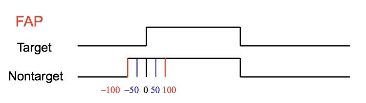
### Focused Attention Paradigm
##############################

# parameter values
# stimulus onset asynchrony
soa <- c(-200, -100, -50, 0, 50, 100, 200)

# processing time of visual/auditory stimulus on stage 1
proc.A <- 100       # = 1/lambdaA
proc.V <- 50

# mean processing time and sd on stage 2
mu <- 150
sigma <- 25

# width of the time window of integration
omega <- 200

# size of cross-modal interaction effect
delta <- 50

# number of observations per SOA
N <- 500

# FAP simulation
data <- simulate.fap(soa, proc.A, proc.V, mu, sigma, omega, delta, N)

# FAP estimation
est <- estimate(data, paradigm = "fap")

# Plot estimates
plotPredObs.fap(data, est)

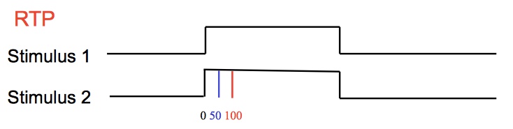
### Redundant Target Paradigm
#############################

# parameter values
# stimulus onset asynchrony
soa <- c(0, 50, 100, 200)

# processing time of visual/auditory stimulus on stage 1
proc.A <- 150       # = 1/lambdaA
proc.V <- 100

# mean processing time and sd on stage 2
mu <- 200
sigma <- mu/5

# width of the time window of integration
omega <- 200

# size of cross-modal interaction effect
delta <- 50

# number of observations per SOA
N <- 500

# RTP simulation
data <- simulate.rtp(soa, proc.A, proc.V, mu, sigma, omega, delta, N)

# RTP estimation
est <- estimate(data, paradigm = "rtp")

# Plot estimates
plotPredObs.rtp(data, est)

# check if predictions are alright
pred <- predict.rt.rtp(c(proc.A, proc.V, mu, omega, delta), colnames(data))

### Estimation Tab Plots ###

# Plot predicted and observed RTs for FAP
plotPredObs.fap <- function(data, est) {

    # get SOA's
    soa <- as.numeric(sub("neg", "-", sub("SOA.", "", colnames(data))))

    # predict RTs from estimations
    pred <- predict.rt.fap(par = est$est$par, column.names = colnames(data))

    # mean and SE of observed reaction times
    obs <- colMeans(data)
    obs_se <- apply(data, 2, sd)/sqrt(nrow(data))

    # plot observed RTs
    plot(obs ~ soa, type="p", col="darkred", xlab="SOA",
         ylab="Reaction time (ms)", xaxt="n",
         ylim=c(min(obs-obs_se), max(obs+obs_se)))
    axis(1, at=soa)

    # add SE
    arrows(soa, obs-obs_se, soa, obs+obs_se, code=3, length=0.02, angle = 90,
           col="darkred")

    # plot predicted RTs
    points(pred ~ soa, type="l")

    legend("bottomright", legend=c("Mean observed RT (+- SE)",
                                   "Mean predicted RT"),
           lty=0:1, pch=c(1, NA), col=c("darkred", "black"))

}


# Plot predicted and observed RTs for RTP
plotPredObs.rtp <- function(data, est) {

    # get SOA's
    soa <- as.numeric(unlist(regmatches(colnames(data),
                                 gregexpr('\\(?[0-9]+',
                                          colnames(data)))))

    # predict RTs from estimations
    pred <- predict.rt.rtp(par = est$est$par, column.names = colnames(data))
    idx.aud <- grep("aud", colnames(data))
    idx.vis <- grep("vis", colnames(data))

    # mean and SE of observed reaction times
    obs <- colMeans(data)
    obs_se <- apply(data, 2, sd)/sqrt(nrow(data))

    # plot observed RTs
    par(mfrow=c(1,2))

    for (first in c("aud", "vis")) {

        if (first == "aud") {
            idx <- idx.aud
            title <- "auditory stimulus first"
        } else if (first == "vis") {
            idx <- idx.vis
            title <- "visual stimulus first"
        }

        plot(obs[idx] ~ soa[idx], type="p", col="darkred", xlab="SOA",
             ylab="Reaction time (ms)", xaxt="n",
             ylim=c(min(obs[idx]-obs_se[idx], pred[idx]),
                    max(obs[idx]+obs_se[idx], pred[idx])),
            main = title)
        axis(1, at=soa)

        # add SE
        arrows(soa[idx], obs[idx]-obs_se[idx], soa[idx],
               obs[idx]+obs_se[idx], code=3, length=0.02, angle = 90,
               col="darkred")

        # plot predicted RTs
        points(pred[idx] ~ soa[idx], type="l")

        legend("bottomright", legend=c("Mean observed RT (+- SE)",
                                       "Mean predicted RT"),
               lty=0:1, pch=c(1, NA), col=c("darkred", "black"))
    }

}

source("simulateFAP.R")
source("simulateRTP.R")
source("estimate.R")
source("plotHelpers.R")

server <- shinyServer(function(input, output, session) {

  ########################
  ### Introduction Tab ###
  ########################

  # Action Buttons that redirect you to the corresponding tab
  observeEvent(input$theorybutton, {
    updateNavbarPage(session, "page", selected = "Theory")
  })

  observeEvent(input$parambutton, {
    updateNavbarPage(session, "page", selected = "Para")
  })

  observeEvent(input$simbutton, {
    updateNavbarPage(session, "page", selected = "Sim")
  })

  observeEvent(input$estbutton, {
    updateNavbarPage(session, "page", selected = "Est")
  })

  ######################
  ### Parameters Tab ###
  ######################

  ### Plot distribution of first stage ###
  output$uni_data_t <- renderPlot({

    # x-sequence for plotting the unimodal distributions
    x <- seq(0,300)

    if (input$distPar == "expFAP") {
      density.t <- dexp(x, rate=1/input$mu_t)
      density.nt <- dexp(x, rate=1/input$mu_nt)
    } else if (input$distPar == "normFAP") {
      density.t <- dnorm(x, mean=input$mun_s1, sd=input$sd_s1)
      density.nt <- dnorm(x, mean=input$mun_s2, sd=input$sd_s2)
    } else {
    # check if given values make sense (kept it in here because we need an
    # interval. Gives error message )
      validate(
        need(input$range_s1[2] - input$range_s1[1] > 0,
             "Please check your input data for the first stimulus!"),
        need(input$range_s2[2] - input$range_s2[1] > 0,
             "Please check your input data for the second stimulus!")
      )
      density.t <- dunif(x, min=input$range_s1[1], max=input$range_s1[2])
      density.nt <- dunif(x, min=input$range_s2[1], max=input$range_s2[2])
    }
    plot(density.t, type="l", xlim=c(0,300), col="red",
      main="First Stage Processing Time Density Function", xlab="time (ms)",
      ylab="density")
    lines(density.nt, xlim=c(0,300), col="blue")
    legend("topright", c("target stimulus", "nontarget stimulus"), col=c("red", "blue"), lty=1)
  })

  ### Plot simulated RT means as a function of SOA ###

  # different stimulus onsets for the non-target stimulus
  tau <- c(-200 ,-150, -100, -50, -25, 0, 25, 50)
  SOA <- length(tau)
  n <- 1000 # number of simulated observations

  # Simulation of fist stage, depending on chosen distribution
  # target stimulus
  stage1_t <- reactive({
    if (input$distPar == "expFAP") (rexp(n, rate = 1/input$mu_t))
    else if (input$distPar == "normFAP") (rnorm(n, mean = input$mun_s1, sd =
                                             input$sd_s1))
    else (runif(n, min = input$range_s1[1], max = input$range_s1[2]))
  })

  # non-target stimulus
  stage1_nt <- reactive({
    if (input$distPar == "expFAP") (rexp(n, rate = 1/input$mu_nt))
    else if (input$distPar == "normFAP") (rnorm(n, mean = input$mun_s2, sd =
                                             input$sd_s2))
    else (runif(n, min = input$range_s2[1], max = input$range_s2[2]))
  })

  # Simulation of the second stage (assumed normal distribution)
  stage2 <- reactive({
    rnorm(n, mean = input$mu_second, sd = input$sd_second)
  })

  # the matrix where integration is simulated in (later on)
  integration <- matrix(0, nrow = n, ncol = SOA)

  output$data <- renderPlot({
    # check if the input variables make sense for the uniform data


    # unimodal reaction times (first plus second stage, without integration)
    obs_t <- stage1_t() + stage2()

    # integration can only occur if the non-target wins the race
    # and the target falls into the time-window <=> non-target + tau < target

    for(i in 1:SOA){
      integration[,i] <- stage1_t() - (stage1_nt() + tau[i])
    } # > 0 if non-target wins, <= 0 if target wins

    # no integration if target wins (preparation for further calculation)
    integration[integration <= 0] <- Inf

    # probability for integration:
    # if the difference between the two stimuli falls into the time-window,
    # integration occurs

    # matrix with logical entries indicating for each run 
    # whether integration takes place (1) or not (0)
    integration <- as.matrix((integration <= input$omega), mode = "integer")

    # bimodal simulation of the data:
    # first stage RT of the target stimulus, second stage processing time
    # and the amount of integration if integration takes place
    obs_bi <- matrix(0, nrow = n, ncol = SOA)
    obs_bi <- stage1_t() + stage2() - integration*input$delta

    # set negative values to zero
    obs_bi[obs_bi < 0] <- 0

    # calculate the RT means of the simulated data for each SOA
    means <- vector(mode = "integer", length = SOA)
    mean_t <- vector(mode = "integer", length = SOA)
    for (i in 1:SOA){
      means[i] <- mean(obs_bi[,i])
      mean_t[i] <- mean(obs_t)
    }

    # store the results in a data frame
    results <- data.frame(tau, mean_t, means)

    # maximum value of the data frame (as threshold for the plot)
    max <- max(mean_t, means) + 50


    # plot the means against the SOA values
    plot(results$tau, results$means, type = "b", col = "red", ylim=c(0, max),
         ylab = "reaction times (ms)", xlab = "stimulus-onset asynchrony (SOA)",
         main = "Mean Predicted Reaction Times for the \nUnimodal and Crossmodal Condition")
    points(results$tau, results$mean_t, type = "l", col = "blue")
    legend("bottomright", title="Condition",
           legend=c("crossmodal", "unimodal"), col=c("red", "blue"), lty=1)
  })

  ### Plot probability of integration as a function of SOA
  # check the input data of the uniform distribution
  output$prob <- renderPlot({

    # same integration calculation as for the other plot
    for (i in 1:SOA) {
      integration[,i] <- stage1_t() - (stage1_nt() + tau[i])
    }
    integration[integration <= 0] <- Inf
    integration <- as.matrix((integration <= input$omega), mode = "integer")

    # calculate the probability for each SOA that integration takes place
    prob_value <- vector(mode = "integer", length = SOA)
    for (i in 1:SOA) {
      prob_value[i] <- sum(integration[,i]) / length(integration[,i])
      # probability of integration for all runs
    }

    # put the results into a data frame
    results <- data.frame(tau, prob_value)

    # plot the results
    if (input$distPar == "uniFAP" && (input$range_s1[2] == input$range_s1[1] ||
                                      input$range_s2[2] == input$range_s2[1]))
      plot()  # plot nothing if it doesnt make sense (they didnt tick an interval, but a single number)

    else {
      plot(results$tau, results$prob_value, type = "b", col = "blue",
              main = "Probability of Integration as a Function of SOA",
              xlab = "stimulus-onset asynchrony (SOA)",
              ylab = "probability of integration")
    }
  })

  ######################
  ### Simulation Tab ###
  ######################

  # Fix variance on second stage
  sigma <- reactive({
      input$mu / 5
  })

  # Input for SOAs
  output$soa_input <- renderUI({
    if (input$paradigmSim == "fap") {
      default.soa <- "-200,-100,-50,0,50,100,200"
    } else if (input$paradigmSim == "rtp") {
      default.soa <- "0,50,100,200"
    }
    textInput("soa.in","Stimulus onset asynchronies (SOAs, comma delimited)",
              default.soa)
  })


  # Get SOAs from input
  soa <- eventReactive(input$sim_button, {
    validate(need(
    tryCatch(soa <- sort(as.numeric(unlist(strsplit(input$soa.in, ",")))),
             error=function(e){}, warning=function(w){}),
                 "SOA input can not be used. Make sure its only comma-separated numbers."))
    soa
  })

  # Simulate data
  dataset <- eventReactive(input$sim_button, {
    if (input$paradigmSim == "fap") {
      list(data = simulate.fap(soa=soa(), proc.A=input$proc.A,
                               proc.V=input$proc.V, mu=input$mu, sigma=sigma(),
                               omega=input$sim.omega, delta=input$sim.delta,
                               N=input$N),
           paradigm = "fap",
           trueValues = c(proc.A=input$proc.A, proc.V=input$proc.V,
                          mu=input$mu, omega=input$sim.omega,
                          delta=input$sim.delta)
           )
    }
    else if (input$paradigmSim == "rtp") {
      list(data = simulate.rtp(soa=soa(), proc.A=input$proc.A,
                                proc.V=input$proc.V, mu=input$mu,
                                sigma=sigma(), omega=input$sim.omega,
                                delta=input$sim.delta, N=input$N),
           paradigm = "rtp",
           trueValues = c(proc.A=input$proc.A, proc.V=input$proc.V,
                          mu=input$mu, omega=input$sim.omega,
                          delta=input$sim.delta)
        )
    }
  })

  # Show data in a table
  output$simtable <- renderTable({
      head(dataset()$data, input$nrowShow)
    })

  # Plot data
  output$simplot <- renderPlot({
      if (dataset()$paradigm == "fap") {
        boxplot(dataset()$data, ylab="reaction time (ms)",
                xlab="stimulus-onset asynchrony (soa)", main="", xaxt="n")
        axis(1, at=1:length(soa()), labels=soa())
      } else if (dataset()$paradigm == "rtp"){
        par(mfrow=c(1,2))
        boxplot(dataset()$data[ , grep("aud", colnames(dataset()$data))],
                ylab="reaction time (ms)", xlab="stimulus-onset asynchrony (soa)",
                main="auditory target", xaxt="n")
        axis(1, at=1:length(soa()), labels=soa())
        boxplot(dataset()$data[ , grep("vis", colnames(dataset()$data))],
                ylab="reaction time (ms)", xlab="stimulus-onset asynchrony (soa)",
                main="visual target", xaxt="n")
        axis(1, at=1:length(soa()), labels=soa())
      }
  })

  # Download the Simulation output

  # downloadHandler() takes two arguments, both functions.
  # The content function is passed a filename as an argument, and
  #   it should write out data to that filename.
  output$downloadData <- downloadHandler(

    # This function returns a string which tells the client
    # browser what name to use when saving the file.
    filename = function() {
      paste("dat-", Sys.Date(), ".csv", sep="")
    },

    # This function should write data to a file given to it by
    # the argument 'file'.
    content = function(file) {
        write.table(dataset()$data, file, quote = FALSE, sep = ";",
                  row.names = FALSE)
    }
  )

  ###################### ESTIMATION ###########################

  correct_colnames <- function(column.names, paradigm) {
    if (paradigm == "rtp") {
      first.stimulus <- unlist(strsplit(column.names, "SOA."))[1]
      suppressWarnings(
        # as.numeric introduces NA, this warning is suppressed
        tau <- as.numeric(unlist(strsplit(column.names, "SOA.")))[2])
      if ((first.stimulus == "aud" | first.stimulus == "vis") &
           !is.na(tau)) {
        NULL
      } else {
        "Did you choose the right paradigm? Column names must be in the form of
        'audSOA.0'. See column names in Simulation tab."
      }
    } else if (paradigm == "fap") {
      suppressWarnings(
        soa <- as.numeric(sub("neg", "-", sub("SOA.", "", column.names))))
        # as.numeric creates NA, this warning is suppressed
      if (!any(is.na(soa))) {
        NULL
      } else {
        "Did you choose the right paradigm? Column names must be in the form of
        'SOA.neg50' or 'SOA.50'. See column names in Simulation tab."
      }
    }
  }

  # Upload data file
  dataUpload <- reactive({
    inFile <- input$file1
    if (is.null(inFile)) return(NULL)
    # read in file
    validate(need(tryCatch(
      data <- read.table(inFile$datapath, header=TRUE, sep=";"),
      error=function(e) {}, warning=function(w) {}),
      "File could not be read in. Make sure it meets the requirements."))

    out <- list(
      data = data,
      paradigm = input$paradigmUpload,
      trueValues = FALSE)

    validate(correct_colnames(colnames(out$data), out$paradigm))
    out
  })

  datasetEst <- reactive({
    if (input$whichDataEst == "sim") {
      # why does this not show?
      validate(need(dataset(), "Simulate data first"))
      dataset()
    }
    else {
      validate(need(dataUpload(), "Upload data first"))
      dataUpload()
    }
  })

  # Estimate parameters according to paradigm
  est.out <- eventReactive(input$est_button, {
    estimate(datasetEst()$data, paradigm=datasetEst()$paradigm)
  })

  # Show parameter estimates
  estTab <- eventReactive(input$est_button, {
    est <- est.out()
      tab <- rbind(round(est$est$par, digits=2),
                   round(est$param.start, digits=2),
                   datasetEst()$trueValues)

      dimnames(tab) <- list(c("estimated value", "start value", "true value"),
                            c("1&#8260&#955<sub>A</sub>",
                              "1&#8260&#955<sub>B</sub>", "&#956", "&#969",
                              "&#948"))

    suppressWarnings( if (datasetEst()$trueValues == FALSE) {
        tab <- tab[1:2,]
    })

      tab
  })

  output$estTextOut <- renderTable({
      estTab()
  }, rownames=TRUE, sanitize.text.function=function(x) x)

  output$chisqValue <- renderTable({
      paste("Objective function value: &#967<sup>2</sup> = ",
            signif(est.out()$est$value, digits=4))
  }, colnames=FALSE, sanitize.text.function=function(x) x)

  # Plot predicted and observed RTs as a function of SOA
  predObsPlot <- eventReactive(input$est_button, {
    est <- est.out()
    if (datasetEst()$paradigm == "fap") {
        plotPredObs.fap(datasetEst()$data, est)
    } else if (datasetEst()$paradigm == "rtp") {
        plotPredObs.rtp(datasetEst()$data, est)
    }
    })

  output$plotPredObs <- renderPlot({
    predObsPlot()
  })
})

##################
### Simulation ###
##################

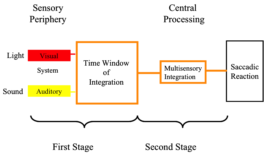
simulate.fap <- function(soa, proc.A, proc.V, mu, sigma, omega, delta, N) {

  # draw random samples for processing time on stage 1 (A and V) or 2 (M)
  nsoa <- length(soa)
  A <- matrix(rexp(N * nsoa, rate = 1/proc.A), ncol = nsoa)
  V <- matrix(rexp(N * nsoa, rate = 1/proc.V), ncol = nsoa)
  M <- matrix(rnorm(N * nsoa, mean = mu, sd = sigma), ncol = nsoa)
  names <- sub("-", "neg", paste0("SOA.", soa))
  dimnames <- list(c(1:N), names)

  data <- matrix(nrow=N, ncol=nsoa,  dimnames= dimnames)

  for (i in 1:N) {
    for(j in 1:nsoa) {
      # is integration happening or not?
      # integration occurs only if (a) the auditory stimulus wins the race in
        # the first stage opening the time window of integration, such that (b)
        # the termination of the visual peripheral process falls into the
        # window (Kandil, Diederich, & Colonius, 2014)
        # I = { A + tau < V < A + tau + omega }
      if (((soa[j] + A[i,j]) < V[i,j]) &&
        (V[i,j] < (soa[j] + A[i,j] + omega))) {
          data[i,j] <- V[i,j] + M[i,j] - delta
      } else
          data[i,j] <- V[i,j] + M[i,j]
  }}

  return(data)
}

##################
### Simulation ###
##################

simulate.first.modality <- function(label, soa, proc.first, proc.second, mu, sigma, omega,
                              delta, N) {
  nsoa <- length(soa)

  # draw random samples for processing time on stage 1 (both modalities) or 2 (M)
  first <- matrix(rexp(N * nsoa, rate = 1/proc.first), ncol = nsoa)
  second <- matrix(rexp(N * nsoa, rate = 1/proc.second), ncol = nsoa)
  M <- matrix(rnorm(N * nsoa, mean = mu, sd = sigma), ncol = nsoa)

  names <- paste0("SOA.", soa)

  # empty data matrix for RTs
  data <- matrix(nrow = N, ncol = nsoa)
  colnames(data) <- paste0(label, names)

  for (i in 1:N) {
    for(j in 1:nsoa) {
      # is integration happening or not?
      if (max(first[i,j], second[i,j] + soa[j]) < min(second[i,j] + soa[j],
                                                      first[i,j]) + omega) {
        data[i,j] <- first[i,j] + M[i,j] - delta
      } else
        data[i,j] <- first[i,j] + M[i,j]
    }}

  return(data)
}

simulate.rtp <- function(soa, proc.A, proc.V, mu, sigma, omega, delta, N) {

  return(
         cbind(auditory = simulate.first.modality(label = "aud", soa,
                                                   proc.first = proc.A,
                                                   proc.second = proc.V, mu,
                                                   sigma, omega, delta, N),
                visual   = simulate.first.modality(label = "vis", soa,
                                                   proc.first = proc.V,
                                                   proc.second = proc.A, mu,
                                                   sigma, omega, delta, N)
            )
         )
}

library(shiny)
library(shinyBS)

shinyUI(
  navbarPage(title = "TWIN Model", theme = "style.css", id = "page",
    ########################
    ### Introduction Tab ###
    ########################

    tabPanel("Introduction", value = "intro",
      withMathJax(),
      tags$head(tags$script(HTML('
        var fakeClick = function(tabName) {
          var dropdownList = document.getElementsByTagName("a");
          for (var i = 0; i < dropdownList.length; i++) {
            var link = dropdownList[i];
            if(link.getAttribute("data-value") == tabName) {
              link.click();
            };
          }
        };
      '))),
      includeScript("../../../Matomo-tquant.js"),
      h2("The Time-Window of Integration Model (TWIN)", align = "center"),
      p("This Shiny App helps you to learn about the Time-Window of
        Integration Model (TWIN), developed by Hans Colonius, Adele Diederich,
        and colleagues", align = "center",
        a("(Colonius & Diederich, 2004).",
          onclick="fakeClick('References')")),
      p("It allows you to visualize model predictions, simulate data, and
        estimate the model parameters either from simulated data or from your
        own datafile.", align = "center"),
      # define action buttons, using raw html. Redirecting doesnt work in CSS
        # because of reasons. ;)
      fluidRow(
        column(3, offset=3,
      actionButton("theorybutton",
        HTML("<strong>Theory</strong><br><p> To learn about the theoretical
             <br> background of the experimental <br> paradigms and the TWIN model
             </p>"),icon("book"), style = "background-color: #ffff99",
             width="300px")),
        column(3,
      actionButton("parambutton",
        HTML("<strong>Parameters</strong><br><p> To play around and visualize
             <br> the model predictions of <br> the Focused Attention Paradigm
             </p>"), icon("area-chart"), style = "background-color: #5fdc5f",
             width="300px"))),
      fluidRow(
        column(3, offset=3,
      actionButton("simbutton",
        HTML("<strong>Simulation</strong> <br><p>To simulate virtual data using
             different <br> parameter values for both <br>
             paradigms</p>"), icon("dashboard"), style="background-color:
             #ed3f40",width="300px")),
        column(3,
      actionButton("estbutton",
        HTML("<strong>Estimation</strong> <br> <p>To estimate the parameters
             either from <br> previously created data (simulation), <br> or
             your own data</p>"), icon("paper-plane"), style="background-color:
             #2f84ff", width="300px"))),
        # adding footer: <div class="footer">Footer text</div>
        tags$div(class = "footer",
          fluidRow(
          column(6,
            p(class="text-info", "This project is part of",
              a(href="https://tquant.eu/", target="_blank",
             img(src="tquant100.png", width = "30%")), align="left")),
          column(6,
                 p("Contact us on", a(icon("github"),"Github",
                   href ="https://github.com/Kaanwoj/shinyTWIN"))))
    )),

      source(file.path("ui", "ui_Theory.R"), local = TRUE)$value,

    ######################
    ### Parameters Tab ###
    ######################

    source(file.path("ui", "ui_Parameters.R"), local = TRUE)$value,

    ######################
    ### Simulation Tab ###
    ######################

    source(file.path("ui", "ui_Simulation.R"), local = TRUE)$value,

    ######################
    ### Estimation Tab ###
    ######################

    source(file.path("ui", "ui_Estimation.R"), local = TRUE)$value,

    source(file.path("ui", "ui_Team.R"), local = TRUE)$value,
    source(file.path("ui", "ui_References.R"), local = TRUE)$value
))

/*-------------------------
	Navbar Customization
--------------------------*/
ul {
   
}

li a {
    color: #666;
}

 a:hover { 
border-bottom: 1px solid #0000FF;
text-decoration: none; 
 }

/*-------------------------
	Buttons
--------------------------*/
 
 
 /*.button {
	background-color: #D5D5D5; 
    border: none;
    color: black;
    padding: 15px 32px;
    text-align: center;
	box-shadow: 0 8px 16px 0 rgba(0,0,0,0.2), 0 6px 20px 0 rgba(0,0,0,0.19);
    text-decoration: none;
    display: inline-block;
    font-size: 16px;
	margin-right:30px;
	
}

/*-------------------------
	Footer
--------------------------*/
.footer {
  position: fixed;
  right: 0;
  bottom: 0;
  left: 0;
  padding: 1rem;
  background-color: #efefef;
  text-align: right;
}
/*-------------------------
	Help Tip
--------------------------*/


.help-tip{
	position: absolute;
	top: 18px;
	right: 18px;
	text-align: center;
	background-color: #BCDBEA;
	border-radius: 50%;
	width: 24px;
	height: 24px;
	font-size: 14px;
	line-height: 26px;
	cursor: default;
}

.help-tip:before{
	content:'?';
	font-weight: bold;
	color:#fff;
}

.help-tip:hover p{
	display:block;
	transform-origin: 100% 0%;

	-webkit-animation: fadeIn 0.3s ease-in-out;
	animation: fadeIn 0.3s ease-in-out;
	 z-index: 999;

}

.help-tip p{
	display: none;
	text-align: left;
	background-color: #1E2021;
	padding: 20px;
	width: 300px;
	position: absolute;
	border-radius: 3px;
	box-shadow: 1px 1px 1px rgba(0, 0, 0, 0.2);
	right: -4px;
	color: #FFF;
	font-size: 13px;
	line-height: 1.4;
}

.help-tip p:before{
	position: absolute;
	content: '';
	width:0;
	height: 0;
	border:6px solid transparent;
	border-bottom-color:#1E2021;
	right:10px;
	top:-12px;
}

.help-tip p:after{
	width:100%;
	height:40px;
	content:'';
	position: absolute;
	top:-40px;
	left:0;
}

@-webkit-keyframes fadeIn {
	0% { 
		opacity:0; 
		transform: scale(0.6);
	}

	100% {
		opacity:100%;
		transform: scale(1);
	}
}

@keyframes fadeIn {
	0% { opacity:0; }
	100% { opacity:100%; }
}

/*------------------------------------
	Vertical Line for Glossary
-------------------------------------*/

.verticalLine {
  border-left: thick solid #ff0000;
}