Introduction
Welcome!
Hello and welcome to this introduction on Item Response Theory, or IRT. IRT is used with testing, to help with item selection and test validation.
In this tutorial, you will:
- Learn the main parameters, models, and assumptions associated with IRT;
- Visualize how changing these parameters affects the models and test;
- Understand how IRT can help identify item biases;
- Learn and test out the relevant R code to fit IRT models.
There will be questions throughout the tutorial, so you can check if you’ve understood the concepts.
Good luck!
Difficulty
Imagine you’re trying to learn someone’s specific ability - for now, let’s take 2nd grade math ability. You develop some questions about math with different levels of difficulty, for example:
- \(4 + 3 = \cdots\)
- \(6 * 7 = \cdots\)
- \(\frac{1}{2} + \frac{1}{4} = \cdots\)
Let’s assume that your questions are directly measuring that person’s ability. If the question has a 50% chance of being answered correctly by a 2nd grader, then you can assume that the difficulty of the item matches the ability of the student: people that answer the question correctly have a higher level of ability than an average 2nd grader, and people that answer incorrectly have a lower level.
This means that the probability that someone correctly responds to a question depends both on that person’s ability and on the difficulty of the question. This is also given by the following model, with ability denoted \(\theta\) and item difficulty denoted \(b_i\). This model is called the Rasch model.
\[P_i(\theta) = \frac{e^{\theta - b_i}}{1 + e^{\theta - b_i}}\]
Experiment with Difficulty
When you plot the probability of someone correctly answering a question depending on their ability, you get an Item Characteristic Curve (ICC), as seen below. To get an idea of how changing the difficulty of the item affects what you can infer about ability, experiment with the difficulty sliders.
Rasch model
The Rasch model only assesses one parameter: difficulty, denoted \(b_i\). As you can see from the graph, the curve for every item can move horizontally, but the shape stays the same. This is because the model assumes that the relation between the item and the latent trait being measured is the same for all items. In practice, however, this relation might vary over the different items. This is why the Two-Parameter Logistic (2PL) model introduces a new parameter: discrimination.
Discrimination
Let’s say that the reason you’re trying to figure out the 2nd grade math ability of a group of kids is because it will determine if certain students will be placed in a remedial math class. You want to make sure that the items are clearly differentiating students that need the remedial class from those who don’t. The discrimination parameter thus shows how well items distinguish between groups. In essence, discrimination measures how well an item relates to the underlying latent ability, so an item that strongly relates to the ability should have a higher discrimination parameter.
Experiment with Discrimination
In the following graph, the difficulties of the three items are set to -2, 0 and 2. Play around with the discrimination to see how the ICCs of these items change.
More about Discrimination
As you can see from the above graph, an item with a higher discrimination has a steeper slope. We can say that such an item discriminates or differentiates better than an item with a lower discrimination and gives more information about someone’s ability. A curious situation occurs when the discrimination is below 0. In that case, people with a lower ability have a higher probability of answering an item correctly than people with a higher ability. This could indicate that an item needs to be rescored, because it was counter-intuitive.
2PL Model:
Adding the discrimination parameter \(a_i\) changes the formula for the probability of a correct response into the Two-Parameter Logistic Model:
\[P_i(\theta) = \frac{e^{a_i (\theta - b_i)}}{1 + e^{a_i (\theta - b_i)}}\]
####Guttman model As you can see when you click the button marked infinity, the discrimination parameter in the 2PL model goes to infinity and the ICC curve becomes deterministic: it fully differentiates between those with higher and lower ability. This version of the 2PL model is called the Guttman model.
Guessing
Almost there! We just need one last ingredient to cover the basics of IRT. So far, as ability decreases, the probability of responding correctly to an item goes towards zero. This means that a person with very low ability will have a near-zero probability of correctly answering the question. But if a question has multiple possible answers, then a person with very low ability can guess one of the possibilities, and so the probability of correctly answering will be larger than zero.
Let’s take an item with four answer options. Without knowing anything about the subject, there is still a 1 in 4 probability of correctly answering the item, given that all options are equally likely. The Three-Parameter Logistic (3PL) model takes this into account by adding a third parameter \(c_i\):
\[P_i(\theta) = c_i + (1 - c_i) \frac{e^{a_i (\theta - b_i)}}{1 + e^{a_i (\theta - b_i)}}\]
Experiment with guessing
In this graph, the difficulty parameters are all equal and the discrimination of all items is set to 1. Pay attention to where the curve hits the y-axis (how the \(P_i(\theta)\) changes) as you change the guessing parameter.
(Note: Although the slider is continuous, the guessing parameter should only take values of 1 divided by the number of questions, such as .5, .25, .33 etc.)
####A note about the 3PL model This model includes a very unlikely assumption: that all answering options are equally likely. This is rarely the case in practice, especially for all participants. This model is thus generally difficult to fit to data.
All 3 parameters
Here you can experiment with all 3 parameters: item difficulty, discrimination and guessing.
Do you understand the IRT parameters?
Assumptions
Like all models, IRT models come with some important assumptions. If these assumptions aren’t met, then the validity and accuracy of the IRT estimates aren’t guaranteed, so you should always keep these assumptions in mind, and check for them when you can.
Unidimensionality
The models we talk about in this tutorial (Rasch, 2PL, 3PL) all assume that the test in question only measures one underlying ability (such as math ability, or \(\theta\)). This means that with the IRT model, we estimate a single \(\theta\) for each student and assume that anything else affecting how students answer questions is just random error.
(Note: multidimensional models do exist, and are used for example with some psychology tests that involve multiple latent traits, but are not covered in this tutorial.)
Local Independence
Once you control for \(\theta\) (e.g., math ability), then there should be no more dependencies between item responses. This means that the only thing different items should have in common is the underlying ability being tested. Local dependencies could occur when multiple questions are based on the same passage or context, for example. To get rid of local dependencies, test creators could drop one of the items, sum the items, or use a model that allows for such dependencies.
Correct Model Specification
The model will only provide accurate estimates of \(\theta\) if the data adheres to the model specifications. For example, if you use a 1PL model to analyze a test with items that have a non-zero asymptote (meaning participants are likely guessing) and that have different slopes (meaning that items discriminate differently with different ability levels), then the model will not fit the data well.
Differential Item Functioning
IRT also can grant insight into how different groups might answer items differently.
Let’s take our 2nd graders again. This time, we have two children of equal ability, both at the average 2nd grade level, answering the same item, which is a word problem about a young boy calculating change. This could produce a “stereotype threat” reaction for a young girl, who has internalized gender-based views on math, causing her to score worse on the item than a young boy, even though they have the same ability level.
Sometimes, people with the same ability but from different groups have different probabilities of correctly answering an item. Only the measured ability is supposed to impact the probability of successfully answering a question, so if there are differences based on group membership, then the test item might be biased. This can be investigated by seeing if there are different ICCs across groups — there can be differences in both difficulty and in discrimination. If an item is labeled with DIF (for Differential Item Functioning), then that item can be removed to attempt to reduce test bias.
Experiment with DIF: Visualization
Here you can see how an item can show a differential functioning unrelated to ability but instead to group differences. For example, let’s say this item assesses intelligence, but it does so differently for 2 groups with the same ability level.
When an item only shows difference in difficulty for different groups, this is called uniform DIF. When the discrimination is also different, this is called non-uniform DIF. It is rare to observe an item with differential discrimination but equivalent difficulty.
TIF & 1PL simulation
So far, we’ve talked about looking at items assessing the ability of one person. In practice, though, IRT is often used to validate questionnaire items, to see what level of ability an item measures and how well it distinguishes between groups. To investigate how test items relate to ability, questionnaires are piloted with a lot of participants, and then the IRT model is fitted to the data.
TIF (Test Information Function)
Now that we have our items and we know how they behave individually, we would like to understand how the test as a whole actually works.
This information is given by the Test Information Function, or TIF. The TIF tells us how well the test assesses the latent trait, or in other words, the precision of the test in measuring a specific level of ability. Precision is the inverse of the variability of the estimated latent trait, so the greater the variability, the less the precision of the test in finding the true value of respondents’ ability.
To help you clearly understand how the characteristics for each item are related to the TIF and the test’s standard error, we’ve provided simulated data for 4 questions, estimated according to a 1PL model.
Model fit
Also make sure you see where the Akaike’s Information Criterion (AIC) and Bayesian Information Criterion (BIC) values are reported. These indices tell us how well the model fits the data, but it’s important to remember that they are comparative indices. This means that to interpret them, you compare the AIC and BIC values from different models, and the model with the smallest values is the best fitting model. This doesn’t mean, however, that the model in question is a good model, just that it fits the data better than the model with larger AIC/BIC values.
When looking at the simulation:
- Try moving around the estimated difficulty of the test and changing its range, then take a look at the graph with the ICCs of each of the four items.
- Compare this to the TIF curve in the graph below, and then look at the standard error. To help you clearly visualize this, we’ve superimposed the TIF and Standard Error (SE) graphs below.
- Notice also how decreasing or increasing the sample size affects the estimated parameters in the above model.
Simulated 1PL data: Difficulty and TIF
Check your understanding of TIF:
2PL simulation
Experiment with the sample size, difficulty and discrimination
This simulated data is modeled with one additional parameter: discrimination. As you saw with the 1PL model on the previous tab, every change in one of the generating parameters affects the estimation of all other parameters. Make sure to observe which changes increase the precision, and which decrease it.
IRT code
We’ll show you a quick sample of some R code, so that you can learn how to fit IRT models to data and make graphs. For demonstration purposes, we’re using a simulated data set of questionnaire responses for 4 items and 500 participants.
(We’re using the ltm package for this tutorial, so
download that package if you want to do similar analyses in R).
library(ltm) #load the ltm package
head(data) #load then inspect your data
## Item 1 Item 2 Item 3 Item 4
## [1,] 1 1 0 0
## [2,] 0 1 0 0
## [3,] 1 0 0 0
## [4,] 1 0 1 0
## [5,] 0 0 0 0
## [6,] 1 0 0 0dim(data) ## [1] 500 4As you can see, this data set shows 4 items with responses from 500 participants. Each response is coded 0 for incorrect and 1 for correct.
Fitting an IRT Model
To fit a 2PL model with varying difficulty and discrimination, use the following code:
IRTmodel = ltm(data ~ z1, IRT.param = TRUE)
coef(IRTmodel)
## Dffclt Dscrmn
## Item 1 -0.01978587 2.7457559
## Item 2 1.05810642 0.6929877
## Item 3 1.40131036 0.9893835
## Item 4 2.76489831 0.7439146Notes on the code:
- The formula
data ~ z1specifies that the data has one latent trait. - The
IRT.param = Tcommand is to ensure correct formatting. coefshows the parameter coefficients
Interpretation: Item 1 has very good discrimination and differentiates best between participants of around average ability (difficulty z-score close to 0). The other items have lower discrimination and best assess ability around 1-2 standard deviations of difficulty above average.
Plotting IRT Models
plot(IRTmodel, type = "ICC", legend=TRUE)
abline(h = .5, lty = 2)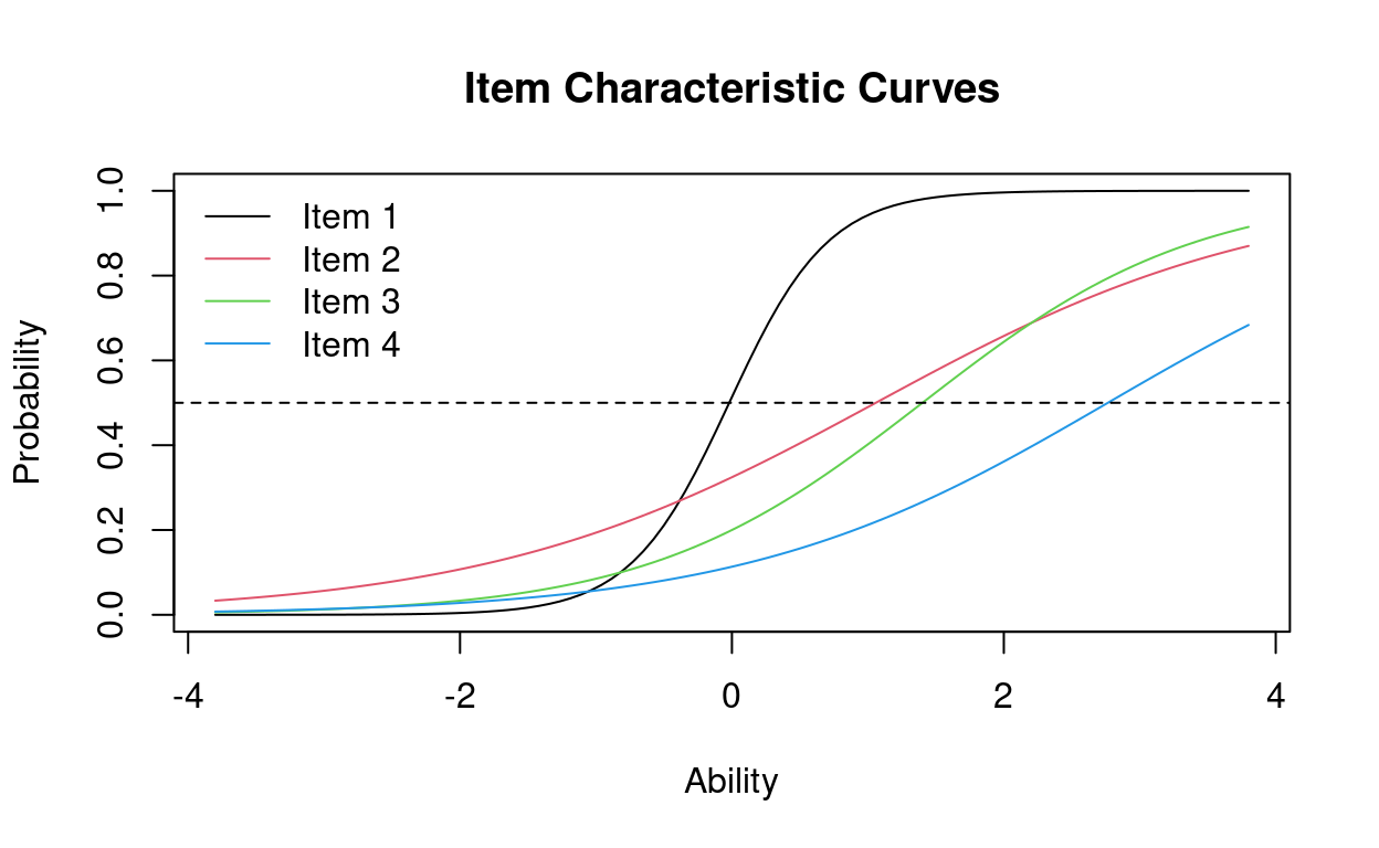
Note: We added a line at P(\(\theta\)) = 0.5, so that we can easily see when an item’s ICC curve crosses this line (i.e., where the item has a 50% chance of being answered correctly). This allows us to assess at a glance an item’s difficulty level.
If you want to just view one item or a select few items, you can use the following code:
plot(IRTmodel, type = "ICC", item = 1)
plot(IRTmodel, type = "ICC", items = c(2,4))
Plotting TIF graphs
To plot the Test Information Function (TIF), use the following code:
plot(IRTmodel, type="IIC", items = 0)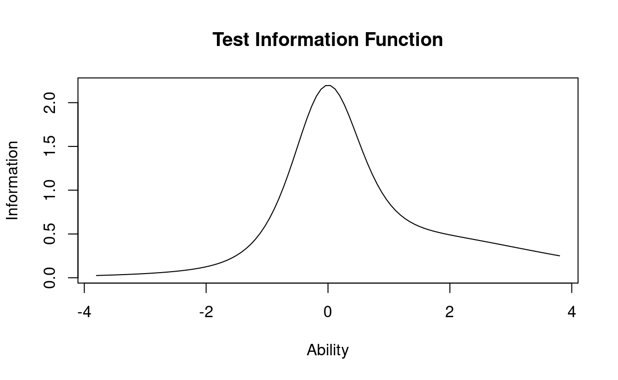
As said before, the TIF reveals where you’re getting the most information about participants. For example, these 4 simulated items gives a lot of information about ability levels near 0.
Other Models & Model Selection
For a 1PL model, with only one parameter that assesses item difficulty, use the following code:
IRTmodel2 = rasch(data)
coef(IRTmodel2)
## Dffclt Dscrmn
## Item 1 -0.02796649 1.062617
## Item 2 0.76631398 1.062617
## Item 3 1.33326793 1.062617
## Item 4 2.10266596 1.062617If you think it’s possible that guessing occurred, you can fit a 3PL model to the data:
IRTmodel3 = tpm(data, type = "latent.trait", IRT.param = T)
coef(IRTmodel3)
## Gussng Dffclt Dscrmn
## Item 1 0.0008239796 -0.006434696 12.478409
## Item 2 0.2055921214 1.471041955 1.474478
## Item 3 0.0765786559 1.530711273 1.320005
## Item 4 0.0813758041 2.017574304 2.251323Model Fit & Model Comparisons
To directly compare two models, you can use the following code:
anova(IRTmodel, IRTmodel3)##
## Likelihood Ratio Table
## AIC BIC log.Lik LRT df p.value
## IRTmodel 2224.19 2257.91 -1104.10
## IRTmodel3 2229.85 2280.42 -1102.92 2.35 4 0.672BIC(IRTmodel) #assesses just the BIC value of one model## [1] 2257.91AIC(IRTmodel3) #assess just the AIC value of one model## [1] 2229.845Compare the AIC/BIC values between two models: the model with the smallest value (as shown above, the 2PL model), is the best fitting model, although the values here are relatively similar.
Code Exercises
Now it’s your turn to try! These code exercises use the
LSAT dataset from the ltm package in R — if
you want to access the dataset from your computer, type
data(LSAT) in your R console.
- Try writing the code on your own first, or by checking the examples from the “IRT coding” page. If you need more help, click on the “Hints” button — the final hint will reveal the solution. Also feel free to play around with the code, and just hit the “Run Code” button when you’re done to see the results.
- See if you can correctly interpret the results by answering the questions below each code exercise.
Load and observe your data
Hint: Try using str(LSAT),
head(LSAT), dim(LSAT) or
descript(LSAT) or any similar functions.
Fitting an IRT model
Fit a 2PL model to the LSAT dataset
LSAT_2pl = LSAT_2pl = ltm(...)LSAT_2pl = ltm(LSAT ~ z1, IRT.param = TRUE)LSAT_2pl = ltm(LSAT ~ z1, IRT.param = TRUE)
coef(LSAT_2pl)Fit a 1PL and a 3PL model to the data
LSAT_1pl =
LSAT_3pl =
LSAT_1pl = rasch(...)
LSAT_3pl = tpm(...)
...
...LSAT_1pl = rasch(LSAT)
LSAT_3pl = tpm(LSAT, type = ..., IRT.param = ...)
coef(...)
coef(...)LSAT_1pl = rasch(LSAT)
LSAT_3pl = tpm(LSAT, type = "latent.trait", IRT.param = T)
coef(LSAT_1pl)
coef(LSAT_3pl)Choosing the best-fitting model
Compare the fit of the 2PL model to the 3PL model
Let’s double check that guessing is an unnecessary parameter.anova(LSAT_2pl, LSAT_3pl) Compare the firt of the 1PL model to the 2PL model
anova(LSAT_1pl, LSAT_2pl) Plotting
Now that we think the 1PL model fits the data well, let’s plot it.
Plot all items from the 2PL model
- Then see if you can plot only items 1 and 5.
plot(LSAT_1pl, type = "ICC") plot(LSAT_1pl, type = "ICC")
abline(h = .5, lty = 2)Plot the TIF function
plot(LSAT_1pl, type="IIC", items = 0)Sources and links
Links:
More info on the
ltmpackage can be found here: https://www.rdocumentation.org/packages/ltmThis tutorial was made with the
learnrpackage for RMarkdown (to learn more, see: https://blog.rstudio.com/2017/07/11/introducing-learnr/).To analyze multidimensional data, the
mirtpackage for R is useful (to learn more, see: https://github.com/philchalmers/mirt/wiki).For a video tutorial on fitting models with the
ltmpackage (that inspired parts of the code questions in this tutorial), see: https://www.youtube.com/watch?v=VtWsyUCGfhg .
Sources:
DeMars, C. (2010). Item response theory: Understanding statistic measurement. New York, NY: Oxford University Press.
This app was developed through the TquanT seminar, by:
M. Annelise Blanchard, University of Leuven, Belgium
Charlotte Tanis, University of Amsterdan, The Netherlands
Ottavia Epifania, University of Padua, Italy