##################
### Estimation ###
##################

# formula (2) in Kandil et al. (2014)
predict.rt <- function(soa, param) {

    lambdaA <- 1/param[1]     # lambdaA
    lambdaV <- 1/param[2]     # lambdaV
    mu      <-   param[3]     # mu
    omega   <-   param[4]     # omega
    delta   <-   param[5]     # delta

    pred <- numeric(length(soa))

    for (i in seq_along(soa)) {

      tau <- soa[i]

      # case 1: tau < tau + omega < 0
      if ((tau <= 0) && (tau + omega < 0)) {
        P.I <- (lambdaV / (lambdaV + lambdaA)) * exp(lambdaA * tau) *
               (-1 + exp(lambdaA * omega))
      }
      # case 2: tau < 0 < tau + omega (should be tau <= 0)
      #         add tau + omega = 0, to include that case here, case 3 would
      #         return Inf
      else if (tau + omega == 0) {
        P.I <- 0
      }
      else if ((tau <= 0) && (tau + omega > 0)) {
        P.I <- 1 / (lambdaV + lambdaA) *
               ( lambdaA * (1 - exp(-lambdaV * (omega + tau))) +
                 lambdaV * (1 - exp(lambdaA * tau)) )
      }
      # case 3: 0 < tau < tau + omega
      else {
        P.I <- (lambdaA / (lambdaV + lambdaA)) *
               (exp(-lambdaV * tau) - exp(-lambdaV * (omega + tau)))
      }
      pred[i] <- 1/lambdaV + mu - delta * P.I
    }

    return(pred)
}

objective.function <- function(param, obs.m, obs.se, soa) {

    # check if parameters are in bounds
    if (param[1] < 5 && param[1] > 250 ) return(60000)  # proc.A
    if (param[2] < 5 && param[2] > 250 ) return(60000)  # proc.A
    if (param[3] < 0                   ) return(60000)  # mu
    if (param[4] < 5 && param[4] > 1000) return(60000)  # omega
    if (param[5] < 0 && param[5] > 175 ) return(60000)  # delta

    pred <- predict.rt(soa, param)

    sum(( (obs.m - pred) / obs.se)^2)
}

estimateFAP <- function(dat, max.iter=100) {

    N <- nrow(dat)

    # Probability of integration
    soa <- c(-200, -100, -50, 0, 50, 100, 200)

    param.start <- c(
                     rexp(1, 1/100),     # proc.A
                     rexp(1, 1/100),     # proc.A
                     rnorm(1, 100, 25),  # mu)
                     rnorm(1, 200, 50),  # omega)
                     rnorm(1, 200, 50)   # delta
                   )

    # observed RTs
    obs.m <- colSums(dat) / N
    obs.se <- apply(dat, 2, sd) / sqrt(N)

    nlm(objective.function, param.start, obs.m = obs.m, obs.se = obs.se, soa
               = soa, iterlim = max.iter)
}
##################
### Estimation ###
##################

# Probability of integration
soa <- c(0, 50, 100, 200)
dat.merge <- cbind(dat.a,dat.v)

# observed RTs
obs.m <- colSums(dat.merge) / N
obs.se <- apply(dat.merge, 2, sd) / sqrt(N)

# predicted RTs

# formula (2) in Kandil et al. (2014)
predict.rt <- function(soa, param) {

    lambdaA <- 1/param[1]
    lambdaV <- 1/param[2]
    mu      <- param[3]
    sigma   <- param[4]
    omega   <- param[5]
    delta   <- param[6]

    predv <- numeric(length(soa))
    preda <- numeric(length(soa))

  # Probability for Integration when the VISUAL stimulus is presented first

    for (i in seq_along(soa)) {

      tau <- soa[i]

      # case 1: visual (=first) wins
      if (tau < omega) {
        P.Iv1 <- 1/(lambdaV+lambdaA) * (lambdaV * (1-exp(lambdaA*(-omega+tau)))+lambdaA*(1-exp(-lambdaV*tau)))
      }
      # case 2: omega <= tau, no integration
      else  {
        P.Iv1 <- lambdaA/(lambdaV+lambdaA)*(exp(-lambdaV*tau)*(-1+exp(lambdaV*omega)))
      }
      # case 3: acoustical (=second) wins, always integration
      P.Iv2 <- lambdaA/(lambdaV+lambdaA)*(exp(-lambdaV*tau)-exp(-lambdaV*(omega+tau)))

      P.Iv = P.Iv1 + P.Iv2

      predv[i] <- 1/lambdaV-exp(-lambdaV*tau)*(1/lambdaV-1/(lambdaV+lambdaA))+ mu - delta * P.Iv
    }
    return(predv)

    # Probability for Integration when the ACOUSTICAL stimulus is presented first

    for (j in seq_along(soa)) {

      tau <- soa[j]

      # case 1: acoustical (=first) wins
      if (tau < omega) {
        P.Ia1 <- 1/(lambdaA+lambdaV) * (lambdaA * (1-exp(lambdaV*(-omega+tau)))+lambdaV*(1-exp(-lambdaA*tau)))
      }
      # case 2: omega <= tau, no integration
      else  {
        P.Ia1 <- lambdaV/(lambdaA+lambdaV)*(exp(-lambdaA*tau)*(-1+exp(lambdaA*omega)))
      }
      # case 3: visual (=second) wins, always integration
      P.Ia2 <- lambdaV/(lambdaV+lambdaA)*(exp(-lambdaA*tau)-exp(-lambdaA*(omega+tau)))

      P.Ia = P.Ia1 + P.Ia2

      preda[j] <- 1/lambdaA-exp(-lambdaA*tau)*(1/lambdaA-1/(lambdaA+lambdaV)) + mu - delta * P.Ia
    }
    return(preda)
    pred.merge <- cbind(preda,predv)
}


objective.function <- function(param, obs.m, obs.se, soa) {

  # check if parameters are in bounds
  if (param[1] < 5 && param[1] > 250 ) return(Inf)  # proc.A
  if (param[2] < 5 && param[2] > 250 ) return(Inf)  # proc.A
  if (param[3] < 0                   ) return(Inf)  # mu
  if (param[4] < 5 && param[4] > 1000) return(Inf)  # omega
  if (param[5] < 0 && param[5] > 175 ) return(Inf)  # delta

  pred.merge <- predict.rt(soa, param)

  sum(( (obs.m - pred.merge) / obs.se)^2)
}

estimateFAP <- function(dat, max.iter=100) {

  N <- nrow(dat)

  # Probability of integration
  soa <- c(0, 50, 100, 200)

  param.start <- c(
    runif(1, 5, 250),   # proc.A
    runif(1, 5, 250),   # proc.A
    runif(1, 0, 1000),  # mu)
    runif(1, 5, 1000),  # omega)
    runif(1, 5, 175)   # delta
  )

  # observed RTs
  obs.m <- colSums(dat) / N
  obs.se <- apply(dat, 2, sd) / sqrt(N)

  nlm(objective.function, param.start, obs.m = obs.m, obs.se = obs.se, soa
      = soa, iterlim = max.iter)
}
source("estimateRTP")
dat.a <- read.table("simDataRTPa.txt", sep=";", header=TRUE)
dat.v <- read.table("simDataRTPv.txt", sep=";", header=TRUE)
estimateRTP(dat.merge)
source("estimateFAP")
dat <- read.table("simDataFAP.txt", sep=";", header=TRUE)
estimateFAP(dat)
library(plyr)
source("simulateFAP.R")
source("estimateFAP.R")
source("simulateRTP.R")
library(xtable)

server <- shinyServer(function(input, output) {

  # different stimulus onsets for the non-target stimulus
  tau <- c(-200 ,-150, -100, -50, -25, 0, 25, 50)
  SOA <- length(tau)
  n <- 1000 # number of simulated observations


  # unimodal simulation of the first stage according to the chosen distribution
  # target stimulus
  stage1_t <- reactive({ if(input$dist == "expFAP")(rexp(n, rate = 1/input$mu_t))
    else (input$dist == "expRSP")(rexp(n, rate = 1/input$mu_t))
  })

  # non-target stimulus
  stage1_nt <- reactive({ if(input$dist == "expFAP")(rexp(n, rate = 1/input$mu_nt))
    else (input$dist == "expRSP")(rexp(n, rate = 1/input$mu_nt))
  })

  # simulation of the second stage (assumed normal distribution)
  stage2 <- reactive({rnorm(n, mean = input$mu_second, sd = input$sd_second)})

  # the matrix where integration is simulated in (later on)
  integration <- matrix(0,
                        nrow = n,
                        ncol = SOA)

  # x-sequence for plotting the unimodeal distributions
  x <- seq(0,300)

  ## --- PLOT THE DISTRIBUTION OF THE FIRST STAGE RT
  output$uni_data_t <- renderPlot({
    # exponential distribution with rate lambda = 1/mu for FAP
    if(input$dist == "expFAP")
      (plot(dexp(x, rate = 1/input$mu_t),
            type = "l",
            lwd=3,
            ylab = "Density Function",
            xlab = "first stage (target stimulus / stimulus 1)"))
    # exp distribution for RSP
    else (input$dist == "expRSP")
    (plot(dexp(x, rate = 1/input$mu_t),
          type = "l",
          lwd=3,
          ylab = "Density Function",
          xlab = "first stage (target stimulus / stimulus 1)"))
  })

  # do the same for the non-target distribution
  output$uni_data_nt <- renderPlot({
    if(input$dist == "expFAP")
      (plot(dexp(x, rate = 1/input$mu_nt),
            type = "l",
            lwd=3,
            ylab = "Density Function",
            xlab = "first stage (non-target stimulus / stimulus 2)"))

    else (input$dist == "expRSP")
    (plot(dexp(x, rate = 1/input$mu_nt),
          type = "l",
          lwd=3,
          ylab = "Density Function",
          xlab = "first stage (non-target stimulus / stimulus 2)"))

  })

  ### --- PLOT THE REACTION TIME MEANS AS FUNCTION OF THE SOA ---
  output$data <- renderPlot({
    # check if the input variables make sense for the uniform data


    # unimodal reaction times (first plus second stage, without integration)
    obs_t <- stage1_t() + stage2()

    # integration can only occur if the non-target wins the race
    # and the target falls into the time-window <=> non-target + tau < target

    for(i in 1:SOA){
      integration[,i] <- stage1_t() - (stage1_nt() + tau[i])
    } # > 0 if non-target wins, <= 0 if target wins

    # no integration if target wins (preparation for further calculation)
    integration[integration <= 0] <- Inf

    # probability for integration:
    # if the difference between the two stimuli falls into the time-window, integration occurs

    # matrix with logical entries indicating for each run
    # whether integration takes place (1) or not (0)
    integration <- as.matrix((integration <= input$omega), mode = "integer")

    # bimodal simulation of the data:
    # first stage RT of the target stimulus, second stage processing time
    # and the amount of integration if integration takes place
    obs_bi <- matrix(0,
                     nrow = n,
                     ncol = SOA)
    obs_bi <- stage1_t() + stage2() - integration*input$delta

    # set negative values to zero
    obs_bi[obs_bi < 0] <- 0

    # calculate the RT means of the simulated data for each SOA
    means <- vector(mode = "integer", length = SOA)
    mean_t <- vector(mode = "integer", length = SOA)
    for (i in 1:SOA){
      means[i] <- mean(obs_bi[,i])
      mean_t[i] <- mean(obs_t)
    }

    # store the results in a data frame
    results <- data.frame(tau, mean_t, means)

    # maximum value of the data frame (as threshold for the plot)
    max <- max(mean_t, means) + 50

    # plot the means against the SOA values
    plot(results$tau, results$means,
         type = "b", col = "red",
         lwd=3,
         ylim=c(0, max),
         ylab = "Reaction Times",
         xlab = "SOA"
         #legend('topright',)
    )
    par(new = T)
    plot(results$tau, results$mean_t,
         type = "l", col = "blue",
         lwd=3,
         ylim = c(0, max),
         ylab = " ",
         xlab = " ")
  })

  ### PLOT THE PROBABILITY OF INTEGRATION ---
  # check the input data of the uniform distribution
  output$prob <- renderPlot({


    # same integration calculation as for the other plot
    for(i in 1:SOA){
      integration[,i] <- stage1_t() - (stage1_nt() + tau[i])
    }
    integration[integration <= 0] <- Inf
    integration <- as.matrix((integration <= input$omega), mode = "integer")

    # calculate the probability for each SOA that integration takes place
    prob_value <- vector(mode = "integer", length = SOA)
    for (i in 1:SOA){
      prob_value[i] <- sum(integration[,i]) / length(integration[,i])
      # probability of integration for all runs
    }

    # put the results into a data frame
    results <- data.frame(tau, prob_value)

    # plot the results
    if(input$dist == "unif" && (input$max_t < input$min_t || input$max_nt < input$min_nt))
      (plot())
    else(plot(results$tau,
              results$prob_value,
              type = "b",
              lwd=3,
              col = "blue",
              ylab = "Probability of Integration",
              xlab = "SOA"))
  })

  output$dt1 <- renderDataTable({
    infile <- input$file1
    if(is.null(infile))
      return(NULL)
    read.csv(infile$datapath, header = TRUE)

  })

  ##################### PDF of article

  output$frame <- renderUI({
    tags$iframe(src="http://jov.arvojournals.org/article.aspx?articleid=2193864.pdf", height=600, width=535)
  })

  ################### Generate the Simulation

  # Simulation with FAP Paradigm
  sigma <- 25
  soa <- reactive({
    if (input$dist2 == "expFAP"){
      soa <- c(-200,-100,-50,0,50,100,200)
    }
     else if (input$dist2 == "expRSP"){
      soa <- rep(c(0,50,100,200), 2)
     }

  })

   dataset <- reactive({
    if (input$dist2 == "expFAP"){
      soa <- c(-200,-100,-50,0,50,100,200)
     simulate.fap (soa, input$proc.A, input$proc.V, input$mu, sigma, input$om, input$del, input$N)
    }
     else if (input$dist2 == "expRSP"){
     soa <- c(0,50,100,200)
     simulate.rtp (soa, input$proc.A, input$proc.V, input$mu, sigma, input$om, input$del, input$N)
     }

  })


  output$simtable <- renderTable(head(dataset(), input$nrowShow))

  output$simplot <- renderPlot({
      plot(colSums(dataset())/input$N, ylab="Reaction time", xlab="SOA",
           main="Mean RT for each SOA", xaxt="n")
      axis(1, at=1:length(soa()), labels=paste0("SOA", soa()))
  })


  ################### Download the Simulation output

  #output$table <- renderTable({
  #data
  #})

  # downloadHandler() takes two arguments, both functions.
  # The content function is passed a filename as an argument, and
  #   it should write out data to that filename.
  output$downloadData <- downloadHandler(

    # This function returns a string which tells the client
    # browser what name to use when saving the file.

    filename = function() {
      #paste(input$dataset, input$filetype, sep = ".")
      paste("dat-", Sys.Date(), ".csv", sep="")
    },

    # This function should write data to a file given to it by
    # the argument 'file'.


    content = function(file) {

      #sep <- switch(input$filetype, "csv" = ",", "tsv" = "\t")

      #write.table(data, file, sep = sep,
      # row.names = FALSE)


      write.csv(dataset(), file)
    }
  )

  ###################### ESTIMATION ###########################
  estimates <- reactive(estimateFAP(dataset()))

  output$estTextOut <- renderTable({
                    est <- matrix(estimates()$estimate, nrow=1)
                    dimnames(est) <- list(NULL, c("1/lambdaA", "1/lambdaV", "mu",
                                                  "omega", "delta"))
                    est
  })


})
##################
### Simulation ###
##################

simulate.fap <- function(soa, proc.A, proc.V, mu, sigma, om, del, N) {

  # draw random samples for processing time on stage 1 (A and V) or 2 (M)
  nsoa <- length(soa)
  A <- matrix(rexp(N * nsoa, rate = proc.A), ncol = nsoa)
  V <- matrix(rexp(N * nsoa, rate = proc.V), ncol = nsoa)
  M <- matrix(rnorm(N * nsoa, mean = mu, sd = sigma), ncol = nsoa)
  dimnames <- list(c(1:N), c("SOA(-200ms)", "SOA(-100ms)","SOA(-50ms)","SOA(0ms)","SOA(50ms)","SOA(100ms)","SOA(-200ms)"))
  data <- matrix(nrow=N, ncol=nsoa,  dimnames= dimnames)

  for (i in 1:N) {
    for(j in 1:nsoa) {
      # is integration happening or not?
      if (((soa[j] + A[i,j]) < V[i,j]) &&
         (V[i,j] < (soa[j] + A[i,j] + om))) {
           data[i,j] <- V[i,j] + M[i,j] - del
      } else
          data[i,j] <- V[i,j] + M[i,j]
  }}
  return(data)

}
##################
### Simulation ###
##################

simulate.rtp <- function(soa, proc.A, proc.V, mu, sigma, omega, delta, N) {

  lambdaA <- 1/proc.A
  lambdaV <- 1/proc.V

  # draw random samples for processing time on stage 1 (only A) or 2 (M)
  nsoa <- length(soa)
  A <- matrix(rexp(N * nsoa, rate = proc.A), ncol = nsoa)
  V <- matrix(rexp(N * nsoa, rate = proc.V), ncol = nsoa)
  M <- matrix(rnorm(N * nsoa, mean = mu, sd = sigma), ncol = nsoa)
  dimnames_a <- list(tr=c(1:N), name=c("SOA(0ms)_A","SOA(50ms)_A","SOA(100ms)_A","SOA(200ms)_A"))
  dimnames_v <- list(tr=c(1:N), name=c("SOA(0ms)_V","SOA(50ms)_V","SOA(100ms)_V","SOA(200ms)_V"))


  data.a <- matrix(nrow=N, ncol=nsoa,dimnames = dimnames_a) # data matrix for RTs

  for (i in 1:N) {
    for(j in 1:nsoa) {
      # is integration happening or not?
      if (max(A[i,j],V[i,j]+soa[j]) < min(V[i,j]+soa[j], A[i,j]) + omega) { # yes
        data.a[i,j] <- A[i,j] + M[i,j] - delta
      } else  # no
        data.a[i,j] <- A[i,j] + M[i,j]
    }}

######## for visual

data.v <- matrix(nrow=N, ncol=nsoa, dimnames = dimnames_v) # data matrix for RTs

for (i in 1:N) {
  for(j in 1:nsoa) {
    # is integration happening or not?
    if (max(A[i,j]+soa[j],V[i,j]) < min(V[i,j], A[i,j]+soa[j]) + omega) {  #yes
      data.v[i,j] <- V[i,j] + M[i,j] - delta
    } else  #no
      data.v[i,j] <- V[i,j] + M[i,j]
  }}
data.merge <- cbind(data.a,data.v)
return(data.merge)


}
##################
### Test cases ###
##################

### RTP simulation
source("simulateRTP.R")

# parameter values
# stimulus onset asynchrony
soa <- c(0, 50, 100, 200)
nsoa <- length(soa)

# processing time of visual/auditory stimulus on stage 1
proc.A <- 100       # = 1/lambdaA
proc.V <- 50

# mean processing time and sd on stage 2
mu <- 150
sigma <- 25

# width of the time window of integration
omega <- 200

# size of cross-modal interaction effect
delta <- 50

# number of observations per SOA
N <- 40

data <- simulate.rtp(soa, proc.A, proc.V, mu, sigma, omega, delta, N)

# save auditory data in a file
df.a <- as.data.frame(data.a)
names(df.a) <- paste0("RTPa", soa)

write.table(df.a, "simDataRTPa.txt", sep=";", row.names=FALSE)

## save visual data in file
df.v <- as.data.frame(data.v)
names(df.v) <- paste0("RTPv", soa)

write.table(df.v, "simDataRTPv.txt", sep=";", row.names=FALSE)
##################
### Test cases ###
##################

### FAP simulation
source("simulateFAP.R")

# parameter values
# stimulus onset asynchrony
soa <- c(-200, -100, -50, 0, 50, 100, 200)


# processing time of visual/auditory stimulus on stage 1
proc.A <- 100       # = 1/lambdaA
proc.V <- 50

# mean processing time and sd on stage 2
mu <- 150
sigma <- 25

# width of the time window of integration
omega <- 200

# size of cross-modal interaction effect
delta <- 50

# number of observations per SOA
N <- 40

data <- simulate.fap(soa, proc.A, proc.V, mu, sigma, omega, delta, N)

# save data in a file
df <- as.data.frame(data)
names(df) <- paste0("FAP", soa)

write.table(df, "simDataFAP.txt", sep=";", row.names=FALSE)
library(shiny)
ui <- shinyUI(
fluidPage(
includeScript("../../../Matomo-tquant.js"),
withMathJax(),
# Application title
fluidRow(
column(6,
img(src = "tquant100.png", align = "left"))),
br(),
headerPanel(h1("The Time-Window of INtegration Model (TWIN)", align = "center")),
h4("Focused Attention Paradigm & Redundant Signals Paradigm", align = "center"),
tabsetPanel(id = "TWINTabset",
tabPanel("Introduction", value = "intro",
fluidRow(
column(4,
wellPanel(
selectInput("topic", "Select the topic: ",
choices = c("About this app" = "aboutapp",
"The TWIN model" = "twinmod",
"Parameters" = "param", "Model equations" = "equ"
)))),
mainPanel(conditionalPanel (condition = ("input.topic == 'aboutapp'"),
p(h2("Welcome!", align = "center")),
br(),
p(h5("This Shiny App helps you to learn more about the Time-Window Ingration Model (TWIN), developed by
Hans Colonius, Adele Diederich, and colleagues.", align = "center")),
p(h5("It allows you to simulate and estimate the parameteres and even to upload your own data file.", align = "center")),
p(h5("Feel free to explore the app and navigate through the tabs!", align ="center")),
br(),
p(h5(strong("Based on the original Shiny App by Annika Thierfelder, this app was expanded by:"), align = "center")),
br(),
p(h5("Aditya Dandekar", img(src="bremen.png", width = "150"),
"Amalia Gomoiu", img(src="glasgow.png", width = "150"), align = "center")),
p(h5("António Fernandes", img(src="lisbon.png", width = "200"),
"Katharina Dücker", img(src="oldenburg.png", width = "110", height = "90"), align = "center")),
p(h5("Katharina Naumann", img(src="tubingen.png", width = "150"),
"Martin Ingram", img(src="glasgow.png", width = "150"), align = "center")),
p(h5("Melanie Spindler", img(src="oldenburg.png", width = "110", height = "90"),
"Silvia Lopes", img(src="lisbon.png", width = "200"), align = "center"))
),
conditionalPanel (condition = ("input.topic == 'twinmod'"),
p(h4("Crossmodal interaction is defined as the situation in which the
perception of an event as measured in terms of one modality
is changed in some way by the concurrent stimulation of one or
more other sensory modalities (Welch & Warren, 1986).", align = "left")),
p(h4("Multisensory integration is defined as the (neural) mechanism underlying
crossmodal interaction.", align = "left")),
p(h4("The Time-Window of Integration Model (TWIN) postulates that a crossmodal
stimulus triggers a race mechanism among the activations in very early,
peripheral sensory pathways. This first stage is followed by a compound
stage of converging subprocesses that comprise neural integration of the
input and preparation of a response. The second stage is defined by
default: It includes all subsequent processes that are not part of the
peripheral processes in the first stage (Diederich, Colonius, & Kandil, 2016).",
align = "left")),
p(img(src="modeltwin.png", width = "550"), align = "center"),
p(h4("At the behavioral level, multisensory integration translates itself into
faster reaction times, higher detection probabilities, and improved discrimination.")),
p(h4("At the neural level, multisensory integration translates itself into an increased total
number of responses, as well as shorter response latencies.")),
p(h4("In the Focused Attention Paradigm (FAP), two or more stimuli are presented
simultaneously or with a short delay between the stimuli.
The participant is asked to respond as quickly as possible
to a stimulus of a pre-defined modality (target) and ignore
the other stimulus (non-target modality).")),
p(img(src="fap.jpeg", width = "500", align = "center")),
p(h4("In the Redundant Signals Paradigm (RSP), two or more stimuli
are also presented simultanously or with a short delay between
the stimulus. However, the participant is asked to respond to
a stimulus of any modality detected first.")),
p(img(src="rtp.jpeg", width = "500", align = "center"))
),
conditionalPanel (condition = ("input.topic == 'param'"),
p(h4("Intensity of the auditory stimuli"), img(src="lamba.jpeg", width = "50"), align = "left"),
p(h4("Intensity of the visual stimuli"), img(src="lambv.jpeg", width = "50"), align = "left"),
p(h4("Processing time for the second stage"), img(src="u.jpeg", width = "40"), align = "left"),
p(h4("Width of the time window of integration"), img(src="w.jpeg", width = "40"), align = "left"),
p(h4("Effect size / Amount of integration"), img(src="delta.jpeg", width = "40"), align = "left")
),
conditionalPanel (condition = ("input.topic == 'equ'"),
p(h4("Requirement for multisensory integration"), img(src="itw.jpeg", width = "300"), align = "left"),
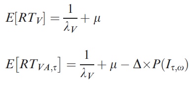
p(h4("Mean reaction times in the unimodal and bimodal conditions"), img(src="rts.jpeg", width = "300"), align = "left"),
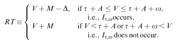
p(h4("Observable reaction time following the logic of the model"), img(src="rt.jpeg", width = "400"), align = "left"),
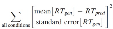
p(h4("Objective function"), img(src="objfun.jpeg", width = "300"), align = "left"),
br(),
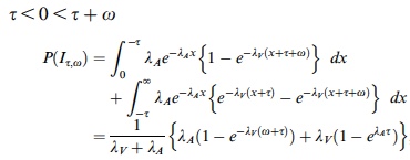
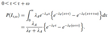
p(h4("Three cases for the probability of integration P(I)")),
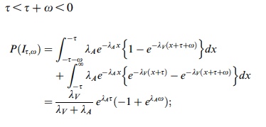
p(img(src="p1.jpeg", width = "400", align = "left")),
p(img(src="p2.jpeg", width = "400", align = "left")),
p(img(src="p3.jpeg", width = "400", align = "left"))
),
br(),
fluidRow(column(8,align="left",
a("Click to learn more", href="http://jov.arvojournals.org/article.aspx?articleid=2193864", target="_blank")
)
)
)
)),
tabPanel("Parameters", value = "Para",
fluidRow(
column(4,
wellPanel(
selectInput("dist", "Distribution ",
choices = c("Exponential" = "expFAP",
" " = "expRSP")),
conditionalPanel( condition = ("input.dist == 'expFAP'"),
sliderInput("mu_t",
"Mean (target / stimulus 1): ",
min = 1,
max = 100,
value = 50),
sliderInput("mu_nt",
"Mean (non-target / stimulus 2): ",
min = 1,
max = 100,
value = 50)
),
conditionalPanel( condition = ("input.dist == 'expRSP'"),
sliderInput("mu_s1",
"Mean (Stimulus 1): ",
min = 1,
max = 100,
value = 50),
sliderInput("mu_s2",
"Mean (Stimulus 2): ",
min = 1,
max = 100,
value = 50)
),
conditionalPanel( condition = ("input.dist == 'normRSP'"),
sliderInput("mun_s1",
"Mean (Stimulus 1): ",
min = 1,
max = 150,
value = 50),
sliderInput("sd_s1",
"Standard deviation (Stimulus 1):",
min = 1,
max = 50,
value = 25),
sliderInput("mun_s2",
"Mean (Stimulus 2): ",
min = 1,
max = 150,
value = 50),
sliderInput("sd_s2",
"Standard Deviation (Stimulus 2):",
min = 1,
max = 50,
value = 25)
),
conditionalPanel( condition = ("input.dist == 'uniRSP'"),
sliderInput("min_s1",
"Minimum (Stimulus 1): ",
min = 1,
max = 300,
value = 50),
sliderInput("max_s1",
"Maximum (Stimulus 1):",
min = 1,
max = 300,
value = 150),
sliderInput("min_s2",
"Minimum (Stimulus 2): ",
min = 1,
max = 300,
value = 50),
sliderInput("max_s2",
"Maximum (Stimulus 2):",
min = 1,
max = 300,
value = 150)
),
sliderInput("mu_second",
"2nd stage processing time: ",
min = 100,
max = 500,
value = 200),
sliderInput("sd_second",
"2nd stage standard deviation:",
min = 0,
max = 100,
value = 50),
sliderInput("delta",
"Amount of Integration: ",
min = -300,
max = 300,
value = 100),
sliderInput("omega",
"Width of the time-window:",
min = 0,
max = 500,
value = 200)
)
),
column(4,
plotOutput("uni_data_t"),
plotOutput("uni_data_nt")),
column(4,
plotOutput("data"),
plotOutput("prob")
)
)),
################### Simulation tab
tabPanel("Simulation", value = "Sim",
#fluidRow(
#column(12,
sidebarLayout(
sidebarPanel(
selectInput("dist2", "Choose paradigm",
choices = c("Focused Attention Paradigm" = "expFAP",
"Redundant Target Paradigm" = "expRSP")),
#conditionalPanel( condition = ("input.dist == 'expFAP'"),
# conditionalPanel( condition = ("input.dist == 'expRSP'"))),
#
h4("First stage"),
sliderInput("proc.A",
"Auditory processing time (\\(\\frac{1}{\\lambda_A}\\))",
min = 20,
max = 150,
value = 100),
sliderInput("proc.V",
"Visual processing time (\\(\\frac{1}{\\lambda_V}\\))",
min = 20,
max = 150,
value = 50),
h4("Second stage"),
sliderInput("mu",
"... processing time (\\(\\mu\\))",
min = 50,
max = 500,
value = 100),
# sliderInput("sigma",
# "Standard Deviation:",
# min = 500,
# max = 200,
# value = 50),
sliderInput("om",
"Window width (\\(\\omega\\))",
min = 100,
max = 300,
value = 200),
sliderInput("del",
"Amount of integration (\\(\\delta\\))",
min = 20,
max = 100,
value = 50),
sliderInput("N",
"Trial Number:",
min = 1,
max = 1000,
value = 500),
downloadButton('downloadData', 'Download (CSV)')
),
mainPanel(
h4("Simulated Data"),
numericInput("nrowShow",
"Number of rows displayed",
min=1,
max=60,
value=10),
tableOutput("simtable"),
plotOutput("simplot")
))
# )
# )
),
tabPanel("Estimation", value = "Est",
fluidRow(
column(4,
wellPanel(
# selectInput("estParadigm", "Chosen Paradigm:",
# choices = c("Focused Attention Paradigm" = "fap",
# "Redundant Signal Paradigm" = "rsp")),
# h4("First stage"),
# sliderInput("est_procV",
# "Visual processing time (\\(\\frac{1}{\\lambda_V}\\))",
# min = 1,
# max = 100,
# value = 50),
# sliderInput("est_procA",
# "Auditory processing time (\\(\\frac{1}{\\lambda_A}\\))",
# min = 1,
# max = 100,
# value = 50),
# h4("Second stage"),
# sliderInput("est_mu",
# "... processing time (\\(\\mu\\))",
# min = 100,
# max = 500,
# value = 50),
# sliderInput("est_omega",
# "Window width (\\(\\omega\\))",
# min = 1,
# max = 100,
# value = 50),
# sliderInput("est_delta",
# "Amount of integration (\\(\\delta\\))",
# min = 1,
# max = 100,
# value = 50),
#actionButton("AButton", "ActionButton"),
#tags$style(HTML('#AButton{background-color:orange}')),
fileInput('file1', 'Choose file to upload',
accept = c(
'text/csv',
'text/comma-separated-values',
'text/tab-separated-values',
'text/plain',
'.csv',
'.tsv'
)
),
fluidRow(column(8,align="left",
a("Click to learn more", href="http://jov.arvojournals.org/article.aspx?articleid=2193864", target="_blank")
)
)
)
),
column(8,
h2("Estimated values"),
tableOutput("estTextOut")
)),
dataTableOutput("dt1")),
#Custom Colored Items
tags$style(HTML(".js-irs-0 .irs-single, .js-irs-0 .irs-bar-edge, .js-irs-0 .irs-bar {background: #000090}")),
tags$style(HTML(".js-irs-1 .irs-single, .js-irs-1 .irs-bar-edge, .js-irs-1 .irs-bar {background: #000070}")),
tags$style(HTML(".js-irs-2 .irs-single, .js-irs-2 .irs-bar-edge, .js-irs-2 .irs-bar {background: #000090}")),
tags$style(HTML(".js-irs-3 .irs-single, .js-irs-3 .irs-bar-edge, .js-irs-3 .irs-bar {background: #000070}")),
tags$style(HTML(".js-irs-4 .irs-single, .js-irs-4 .irs-bar-edge, .js-irs-4 .irs-bar {background: #000090}")),
tags$style(HTML(".js-irs-5 .irs-single, .js-irs-5 .irs-bar-edge, .js-irs-5 .irs-bar {background: #000070}")),
tags$style(HTML(".js-irs-6 .irs-single, .js-irs-6 .irs-bar-edge, .js-irs-6 .irs-bar {background: #000090}")),
tags$style(HTML(".js-irs-7 .irs-single, .js-irs-7 .irs-bar-edge, .js-irs-7 .irs-bar {background: #000070}")),
tags$style(HTML(".js-irs-8 .irs-single, .js-irs-8 .irs-bar-edge, .js-irs-8 .irs-bar {background: #000070}")),
tags$style(HTML(".js-irs-9 .irs-single, .js-irs-9 .irs-bar-edge, .js-irs-9 .irs-bar {background: #000070}")),
tags$style(HTML(".js-irs-10 .irs-single, .js-irs-10 .irs-bar-edge, .js-irs-10 .irs-bar {background: #000070}"))
))
)

 Amalia Gomoiu

 Katharina Dücker

 Martin Ingram